Queueing theory describes the movement of a queue such as customer arrival in bank, shop or emergency department. It seeks to balance supply and demand for a service. It begun with the study queue waiting on Danish telephones in 1909.
Little’s theorem describes the linear relationship between the number of customer L to the customer arrival rate \(\lambda\) and the customer served per time peiod, \(\mu\). This can also be used to determine the number of beds needed for coronary care unit given 4 patients being admitted to cardiology unit, one of whom needs to be admitted to coronary care unit and would stay for an average of 3 days.
Queueing system is described in terms of Kendall’s notation, M/M/c/k, with exponential arrival time. Using this terminology, MM1 system has 1 server and infinite queue. An MM/2/3 system has 2 (c) servers and 1 (k-c) position in the queue. The M refers to Markov chain.
An example of a single server providing full service is a car wash. Example of a single multiphase server include different single stations in bank of withdrawing, deposit, information A counter at the airport or train station for economy and business passengers is considered multiserver single phase queue. A laundromat with different queues for washing and drying is an example of multiphase multiservers.
A traditional queue at a shop can also be seen as first in first out with the first customer served first and leave first. An issue with FIFO is that people may queue early such as overnight queue for the latest iPhone. Alternatives include last in first out queue and priority queueing in emergency department.
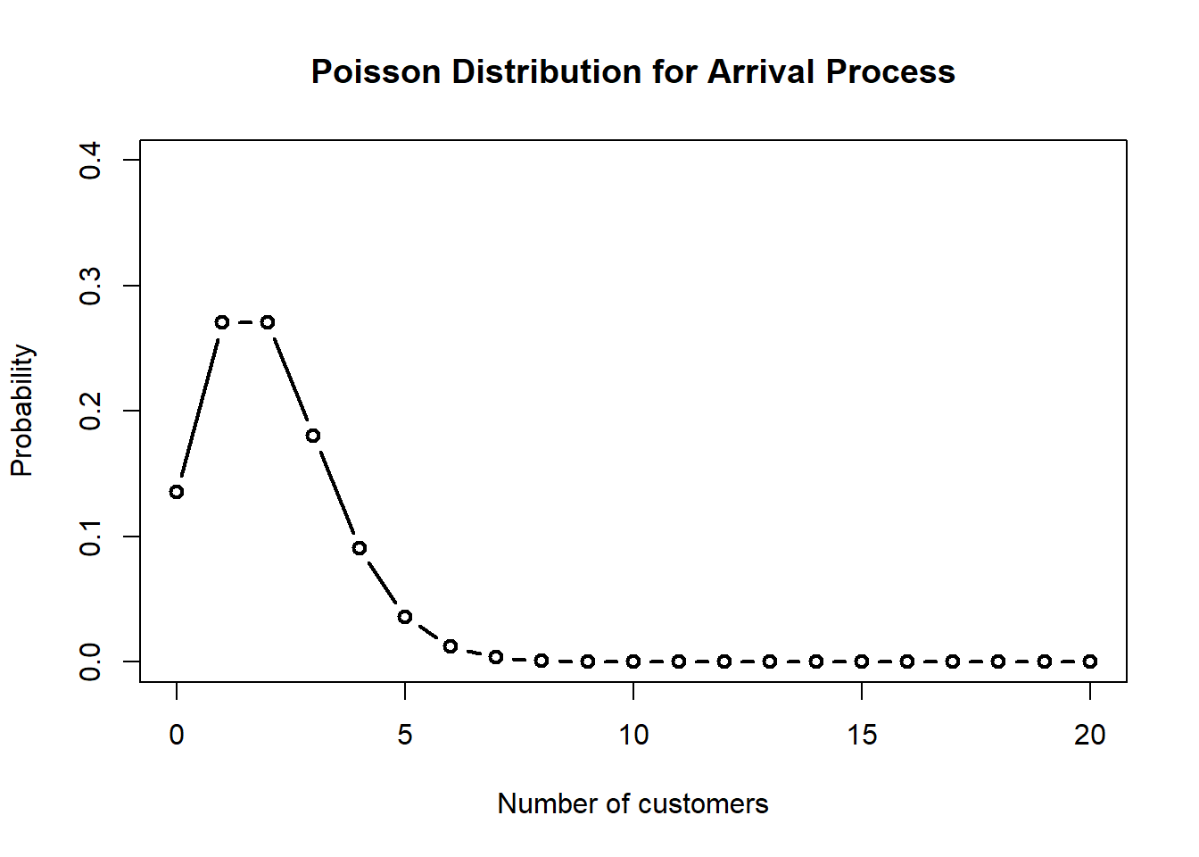
Let’s create a simple queue with 2 customers arriving per minute and 3 customers served per minute. The PO is the probability that the server is idle.
library(queueing)lambda <-2# 2 customers arriving per minutemu <-3# 3 customers served per minute# MM1 mm1 <-NewInput.MM1(lambda =2, mu =3, n =0)# Create queue class objectmm1_out <-QueueingModel(mm1)# ReportReport(mm1_out)
The inputs of the M/M/1 model are:
lambda: 2, mu: 3, n: 0

The outputs of the M/M/1 model are:

The probability (p0, p1, ..., pn) of the n = 0 clients in the system are:
0.3333333
The traffic intensity is: 0.666666666666667
The server use is: 0.666666666666667
The mean number of clients in the system is: 2
The mean number of clients in the queue is: 1.33333333333333
The mean number of clients in the server is: 0.666666666666667
The mean time spend in the system is: 1
The mean time spend in the queue is: 0.666666666666667
The mean time spend in the server is: 0.333333333333333
The mean time spend in the queue when there is queue is: 1
The throughput is: 2
# Summarysummary(mm1_out)
  lambda mu c  k  m        RO        P0       Lq        Wq X L W Wqq Lqq
1      2  3 1 NA NA 0.6666667 0.3333333 1.333333 0.6666667 2 2 1   1   3
curve(dpois(x, mm1$lambda),from =0, to =20, type ="b", lwd =2,xlab ="Number of customers",ylab ="Probability",main ="Poisson Distribution for Arrival Process",ylim =c(0, 0.4),n =21)
Lets examine M/M/3 queue with exponential inter-arrival times, exponential service times and 3 servers.
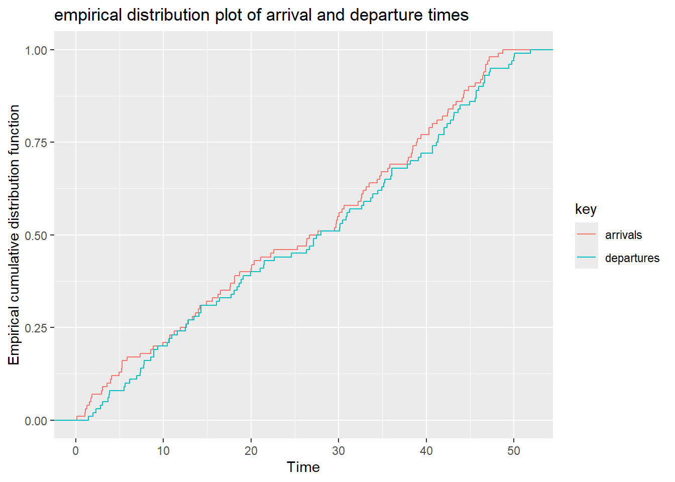
Discrete event simulation can be consider as modeling a complexity of system with multiple processes over time. This is different from continuous modeling of a system which evolve continuously with time. Discrete event simulation can be apply to the study of queue such as bank teller with a first in first out system.
13.2.1 Simulate capacity of system
The example below is a based on examples provided in the simmer website for laundromat.
The following objects are masked from 'package:simmer':

    get_mon_arrivals, get_mon_attributes, get_mon_resources
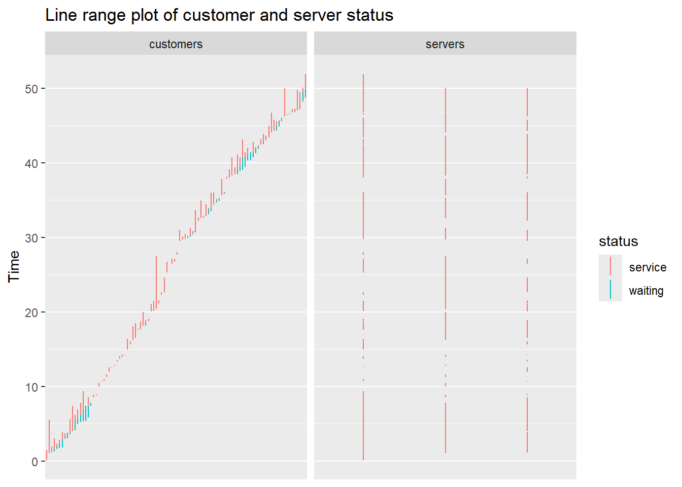
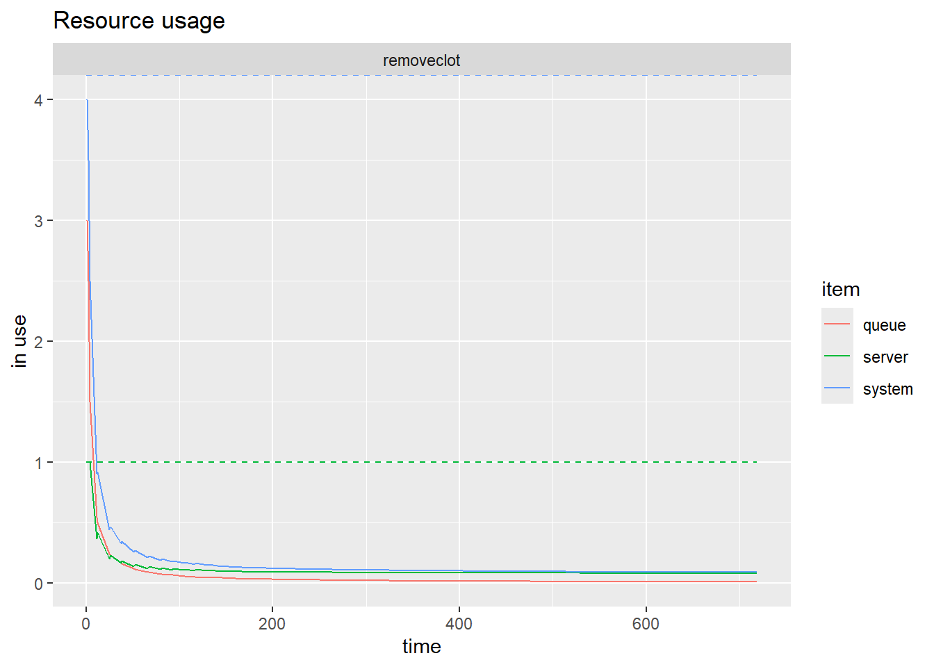
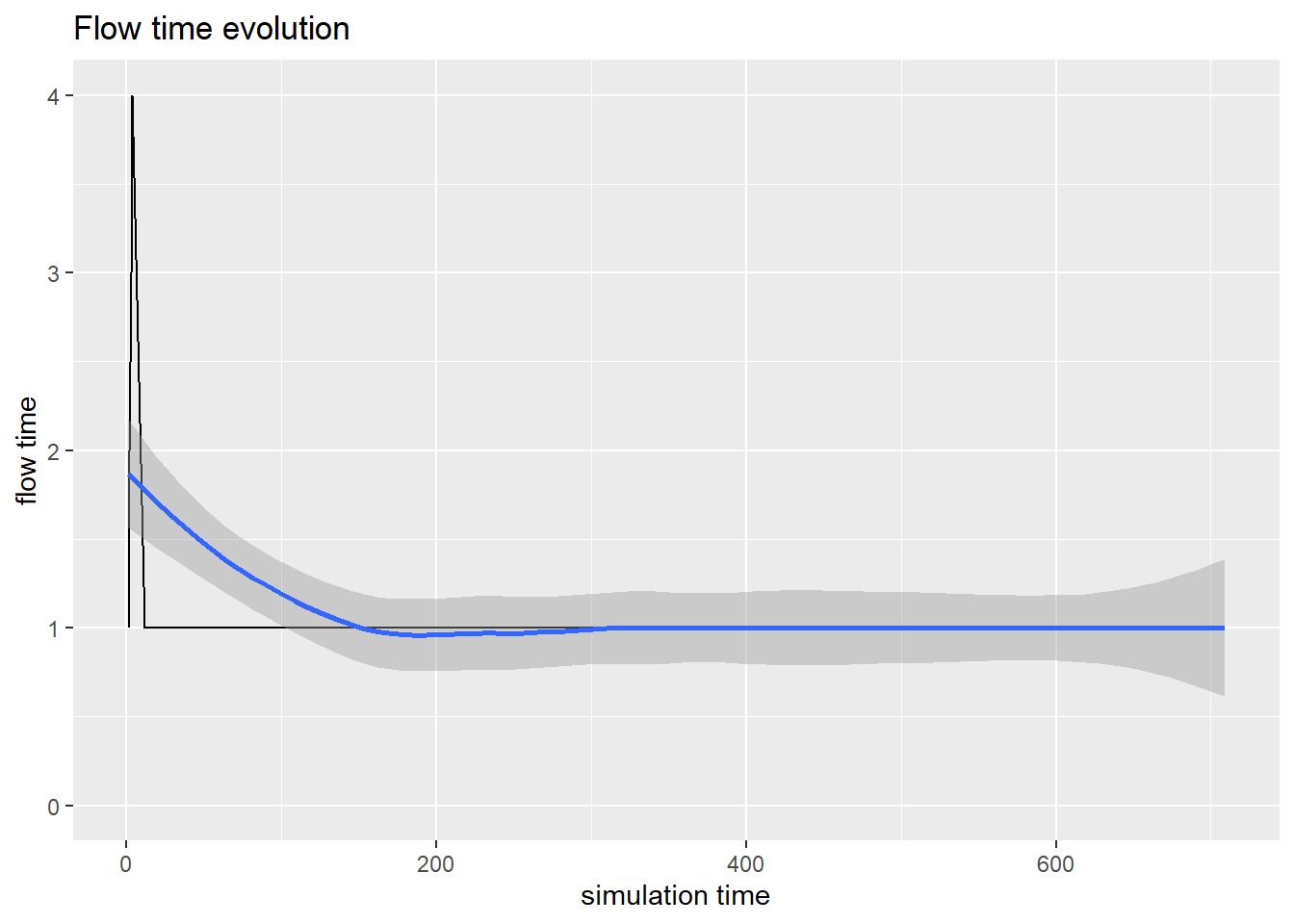
NUM_ANGIO <-1# Number of machines for performing ECRECRTIME <-1# hours it takes to perform ECR~ 90/60T_INTER <-13# new patient every ~365*24/700 hoursSIM_TIME <-24*30# Simulation time over 30 days# setupset.seed(42)env <-simmer()patient <-trajectory() %>%log_("arrives at the ECR") %>%seize("removeclot", 1) %>%log_("enters the ECR") %>%timeout(ECRTIME) %>%set_attribute("clot_removed", function() sample(50:99, 1)) %>%log_(function() paste0(get_attribute(env, "clot_removed"), "% of clot was removed")) %>%release("removeclot", 1) %>%log_("leaves the ECR")env %>%add_resource("removeclot", NUM_ANGIO) %>%# feed the trajectory with 4 initial patientsadd_generator("patient_initial", patient, at(rep(0, 4))) %>%# new patient approx. every T_INTER minutesadd_generator("patient", patient, function() sample((T_INTER-2):(T_INTER+2), 1)) %>%# start the simulationrun(SIM_TIME)
0: patient_initial0: arrives at the ECR
0: patient_initial0: enters the ECR
0: patient_initial1: arrives at the ECR
0: patient_initial2: arrives at the ECR
0: patient_initial3: arrives at the ECR
1: patient_initial0: 86% of clot was removed
1: patient_initial0: leaves the ECR
1: patient_initial1: enters the ECR
2: patient_initial1: 50% of clot was removed
2: patient_initial1: leaves the ECR
2: patient_initial2: enters the ECR
3: patient_initial2: 74% of clot was removed
3: patient_initial2: leaves the ECR
3: patient_initial3: enters the ECR
4: patient_initial3: 59% of clot was removed
4: patient_initial3: leaves the ECR
11: patient0: arrives at the ECR
11: patient0: enters the ECR
12: patient0: 67% of clot was removed
12: patient0: leaves the ECR
25: patient1: arrives at the ECR
25: patient1: enters the ECR
26: patient1: 98% of clot was removed
26: patient1: leaves the ECR
37: patient2: arrives at the ECR
37: patient2: enters the ECR
38: patient2: 74% of clot was removed
38: patient2: leaves the ECR
51: patient3: arrives at the ECR
51: patient3: enters the ECR
52: patient3: 95% of clot was removed
52: patient3: leaves the ECR
66: patient4: arrives at the ECR
66: patient4: enters the ECR
67: patient4: 75% of clot was removed
67: patient4: leaves the ECR
80: patient5: arrives at the ECR
80: patient5: enters the ECR
81: patient5: 96% of clot was removed
81: patient5: leaves the ECR
92: patient6: arrives at the ECR
92: patient6: enters the ECR
93: patient6: 90% of clot was removed
93: patient6: leaves the ECR
105: patient7: arrives at the ECR
105: patient7: enters the ECR
106: patient7: 76% of clot was removed
106: patient7: leaves the ECR
116: patient8: arrives at the ECR
116: patient8: enters the ECR
117: patient8: 86% of clot was removed
117: patient8: leaves the ECR
130: patient9: arrives at the ECR
130: patient9: enters the ECR
131: patient9: 54% of clot was removed
131: patient9: leaves the ECR
145: patient10: arrives at the ECR
145: patient10: enters the ECR
146: patient10: 83% of clot was removed
146: patient10: leaves the ECR
159: patient11: arrives at the ECR
159: patient11: enters the ECR
160: patient11: 89% of clot was removed
160: patient11: leaves the ECR
173: patient12: arrives at the ECR
173: patient12: enters the ECR
174: patient12: 82% of clot was removed
174: patient12: leaves the ECR
186: patient13: arrives at the ECR
186: patient13: enters the ECR
187: patient13: 73% of clot was removed
187: patient13: leaves the ECR
198: patient14: arrives at the ECR
198: patient14: enters the ECR
199: patient14: 64% of clot was removed
199: patient14: leaves the ECR
211: patient15: arrives at the ECR
211: patient15: enters the ECR
212: patient15: 57% of clot was removed
212: patient15: leaves the ECR
223: patient16: arrives at the ECR
223: patient16: enters the ECR
224: patient16: 53% of clot was removed
224: patient16: leaves the ECR
237: patient17: arrives at the ECR
237: patient17: enters the ECR
238: patient17: 94% of clot was removed
238: patient17: leaves the ECR
249: patient18: arrives at the ECR
249: patient18: enters the ECR
250: patient18: 54% of clot was removed
250: patient18: leaves the ECR
263: patient19: arrives at the ECR
263: patient19: enters the ECR
264: patient19: 83% of clot was removed
264: patient19: leaves the ECR
277: patient20: arrives at the ECR
277: patient20: enters the ECR
278: patient20: 84% of clot was removed
278: patient20: leaves the ECR
289: patient21: arrives at the ECR
289: patient21: enters the ECR
290: patient21: 75% of clot was removed
290: patient21: leaves the ECR
300: patient22: arrives at the ECR
300: patient22: enters the ECR
301: patient22: 55% of clot was removed
301: patient22: leaves the ECR
312: patient23: arrives at the ECR
312: patient23: enters the ECR
313: patient23: 52% of clot was removed
313: patient23: leaves the ECR
324: patient24: arrives at the ECR
324: patient24: enters the ECR
325: patient24: 51% of clot was removed
325: patient24: leaves the ECR
339: patient25: arrives at the ECR
339: patient25: enters the ECR
340: patient25: 59% of clot was removed
340: patient25: leaves the ECR
351: patient26: arrives at the ECR
351: patient26: enters the ECR
352: patient26: 82% of clot was removed
352: patient26: leaves the ECR
366: patient27: arrives at the ECR
366: patient27: enters the ECR
367: patient27: 88% of clot was removed
367: patient27: leaves the ECR
377: patient28: arrives at the ECR
377: patient28: enters the ECR
378: patient28: 94% of clot was removed
378: patient28: leaves the ECR
391: patient29: arrives at the ECR
391: patient29: enters the ECR
392: patient29: 58% of clot was removed
392: patient29: leaves the ECR
403: patient30: arrives at the ECR
403: patient30: enters the ECR
404: patient30: 61% of clot was removed
404: patient30: leaves the ECR
418: patient31: arrives at the ECR
418: patient31: enters the ECR
419: patient31: 58% of clot was removed
419: patient31: leaves the ECR
432: patient32: arrives at the ECR
432: patient32: enters the ECR
433: patient32: 84% of clot was removed
433: patient32: leaves the ECR
445: patient33: arrives at the ECR
445: patient33: enters the ECR
446: patient33: 65% of clot was removed
446: patient33: leaves the ECR
460: patient34: arrives at the ECR
460: patient34: enters the ECR
461: patient34: 77% of clot was removed
461: patient34: leaves the ECR
475: patient35: arrives at the ECR
475: patient35: enters the ECR
476: patient35: 77% of clot was removed
476: patient35: leaves the ECR
490: patient36: arrives at the ECR
490: patient36: enters the ECR
491: patient36: 67% of clot was removed
491: patient36: leaves the ECR
502: patient37: arrives at the ECR
502: patient37: enters the ECR
503: patient37: 67% of clot was removed
503: patient37: leaves the ECR
513: patient38: arrives at the ECR
513: patient38: enters the ECR
514: patient38: 95% of clot was removed
514: patient38: leaves the ECR
528: patient39: arrives at the ECR
528: patient39: enters the ECR
529: patient39: 85% of clot was removed
529: patient39: leaves the ECR
543: patient40: arrives at the ECR
543: patient40: enters the ECR
544: patient40: 85% of clot was removed
544: patient40: leaves the ECR
554: patient41: arrives at the ECR
554: patient41: enters the ECR
555: patient41: 67% of clot was removed
555: patient41: leaves the ECR
566: patient42: arrives at the ECR
566: patient42: enters the ECR
567: patient42: 62% of clot was removed
567: patient42: leaves the ECR
579: patient43: arrives at the ECR
579: patient43: enters the ECR
580: patient43: 68% of clot was removed
580: patient43: leaves the ECR
594: patient44: arrives at the ECR
594: patient44: enters the ECR
595: patient44: 78% of clot was removed
595: patient44: leaves the ECR
608: patient45: arrives at the ECR
608: patient45: enters the ECR
609: patient45: 93% of clot was removed
609: patient45: leaves the ECR
619: patient46: arrives at the ECR
619: patient46: enters the ECR
620: patient46: 70% of clot was removed
620: patient46: leaves the ECR
630: patient47: arrives at the ECR
630: patient47: enters the ECR
631: patient47: 97% of clot was removed
631: patient47: leaves the ECR
643: patient48: arrives at the ECR
643: patient48: enters the ECR
644: patient48: 87% of clot was removed
644: patient48: leaves the ECR
658: patient49: arrives at the ECR
658: patient49: enters the ECR
659: patient49: 62% of clot was removed
659: patient49: leaves the ECR
669: patient50: arrives at the ECR
669: patient50: enters the ECR
670: patient50: 58% of clot was removed
670: patient50: leaves the ECR
684: patient51: arrives at the ECR
684: patient51: enters the ECR
685: patient51: 92% of clot was removed
685: patient51: leaves the ECR
696: patient52: arrives at the ECR
696: patient52: enters the ECR
697: patient52: 91% of clot was removed
697: patient52: leaves the ECR
708: patient53: arrives at the ECR
708: patient53: enters the ECR
709: patient53: 78% of clot was removed
709: patient53: leaves the ECR
719: patient54: arrives at the ECR
719: patient54: enters the ECR
`geom_smooth()` using method = 'loess' and formula = 'y ~ x'
Now we will fork another path in the patient flow
13.2.2 Queuing network
mean_pkt_size <-100# byteslambda1 <-2# pkts/slambda3 <-0.5# pkts/slambda4 <-0.6# pkts/srate <-2.2* mean_pkt_size # bytes/s# set an exponential message size of mean mean_pkt_sizeset_msg_size <-function(.)set_attribute(., "size", function() rexp(1, 1/mean_pkt_size))# seize an M/D/1 queue by id; the timeout is function of the message sizemd1 <-function(., id)seize(., paste0("md1_", id), 1) %>%timeout(function() get_attribute(env, "size") / rate) %>%release(paste0("md1_", id), 1)
Linear programming is an optimisation process to maximise profit and minimise cost with multiple parts of the model having linear relationship. There are several different libraries useful for linear programming. The lpSolve library is used here as illustration.
library(lpSolve)#solve using linear programmingn <-2.5# Numbers of techs. 1 EFT means a person is employed for 40 hours a week and 0.5 EFT means a person is employed for 20 hours a week.set_up_eeg <-40# 40 minutesto_do_eeg <-30# 30 minutesclean_equipment <-20# 20 minutesannotate_eeg <-10# 10 minutes# put some error for EEG time# if error=1 that mean NO errors happenerror <-0.8#change from 0.93#Calculate time for EEG in houreeg_case_time <- ((set_up_eeg+to_do_eeg+clean_equipment+annotate_eeg)/60)*error# limit for EEG per day# we can put different limits for EEGslimit_eeg <-round(8*eeg_case_time, digits =0)#s[i] - numbers of cases for each i-EEG's machines #Setting the coefficients of s[i]-decision variables#In a future can put some efficiency or some costobjective.in=c(1,1,1,1,1)#Constraint Matrixconst.mat=matrix(c(1,0,0,0,0,0,1,0,0,0,0,0,1,0,0,0,0,0,1,0,0,0,0,0,1,1,1,1,1,1),nrow =6,byrow = T)#defining constraintsconst_num_1=limit_eeg #in casesconst_num_2=limit_eeg #in casesconst_num_3=limit_eeg #in casesconst_num_4=limit_eeg #in casesconst_num_5=limit_eeg #in casesconst_res= n*7# limit per sessions#RHS for constraintsconst.rhs=c(const_num_1,const_num_2,const_num_3,const_num_4,const_num_5, const_res)#Direction for constraintsconstr.dir <-rep("<=",6)#Finding the optimum solutionopt=lp(direction ="max",objective.in,const.mat,constr.dir,const.rhs)#summary(opt)#Objective values of s[i]opt$solution
[1] 11.0 6.5 0.0 0.0 0.0
Estimate for day (Value of objective function at optimal point)
[1] 17.5
Estimate EEG per month based on staff EFT- only 2.5
[1] 366
Assuming that the time spend on a report by neurologists (1 report = 30 min) then in a 3.5 hour session a neurologist can report 7 EEG.
Forecasting is useful in predicting trends. In health care it can be used for estimating seasonal trends and bed requirement. Below is a forecast of mortality from COVID-19 in 2020. This forecast is an example and is not meant to be used in practice as mortality from COVID depends on the number of factors including infected cases, age, socioeconomic group, and comorbidity.
# A data frame with columns ds & y (datetimes & metrics)covid<-rename(covid, ds =Date, y=Total.Deaths)covid2 <- covid[c(1:12),]m<-prophet(covid2)#create prophet object
Disabling yearly seasonality. Run prophet with yearly.seasonality=TRUE to override this.
Disabling weekly seasonality. Run prophet with weekly.seasonality=TRUE to override this.
Disabling daily seasonality. Run prophet with daily.seasonality=TRUE to override this.
n.changepoints greater than number of observations. Using 8
# Extend dataframe 12 weeks into the futurefuture <-make_future_dataframe(m, freq="week" , periods =26)# Generate forecast for next 500 daysforecast <-predict(m, future)# What's the forecast for July 2020?forecasted_rides <- forecast %>%arrange(desc(ds)) %>% dplyr::slice(1) %>%pull(yhat) %>%round()forecasted_rides
[1] 67488
# Visualizeforecast_p <-plot(m, forecast) +labs(x ="", y ="mortality", title ="Projected COVID-19 world mortality", subtitle ="based on data truncated in January 2020") +ylim(20000,80000)+theme_ipsum_rc()#forecast_p
13.4.1 Bed requirement
13.4.2 Length of stay
13.4.3 Customer churns
Customer churns or turnover is an issue of interest in marketing. The corollary within healthcare is patients attendance at outpatient clinics, Insurance. The classical method used is GLM.
Data from WHO on mortality rate can be extracted directly from WHO or by calling get_who_mr in heemod library.
library(heemod)
Attaching package: 'heemod'
The following object is masked from 'package:purrr':

    modify
The following object is masked from 'package:simmer':

    join
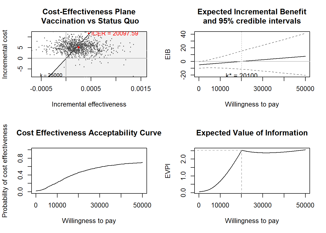
There are several data in BCEA library such as Vaccine.
library(BCEA)
The BCEA version loaded is: 2.4.4
Attaching package: 'BCEA'
The following object is masked from 'package:graphics':

    contour
#use Vaccine data from BCEAdata(Vaccine)ints=c("Standard care","Vaccination")# Runs the health economic evaluation using BCEAm <-bcea(e=eff,c=cost, # defines the variables of # effectiveness and costref=2, # selects the 2nd row of (e, c) # as containing the reference interventioninterventions=treats, # defines the labels to be associated # with each interventionKmax=50000, # maximum value possible for the willingness # to pay threshold; implies that k is chosen # in a grid from the interval (0, Kmax)plot=TRUE# plots the results)