3  Medical Images

3.0.1 DICOM and nifti format

R can handle a variety of different data format. Medical images are stored as DICOM files for handling and converted to nifti files for analysis. The workhorses are the oro.dicom and oro.nifti libraries. Nifti is an S4 class object with multiple slots for data type. These slots can be accessed by typing the @ after the handle of the file. The values in an image can be evaluated using range function. Alternately, use cal_max and cal_min to perform the same task. It appears that in the conversion from minc file to nifti file, a scaling factor has been applied and transformed the values.

library(oro.nifti)

oro.nifti 0.11.4

mca<-readNIfTI("./Data-Use/mca_notpa.nii.gz", reorient = FALSE) 

range(mca)

[1] 0.000000000 0.001411765

The slots also contain information on whether the data has been scaled. This can be checked by accessing the scl_slope and scl_inter slots. These data on slope and intercept provide a mean of returning an image to its correct value.

mca@scl_slope

[1] 1

To find available slots

#find available of slots
slotNames(mca)

 [1] ".Data"          "sizeof_hdr"     "data_type"      "db_name"       
 [5] "extents"        "session_error"  "regular"        "dim_info"      
 [9] "dim_"           "intent_p1"      "intent_p2"      "intent_p3"     
[13] "intent_code"    "datatype"       "bitpix"         "slice_start"   
[17] "pixdim"         "vox_offset"     "scl_slope"      "scl_inter"     
[21] "slice_end"      "slice_code"     "xyzt_units"     "cal_max"       
[25] "cal_min"        "slice_duration" "toffset"        "glmax"         
[29] "glmin"          "descrip"        "aux_file"       "qform_code"    
[33] "sform_code"     "quatern_b"      "quatern_c"      "quatern_d"     
[37] "qoffset_x"      "qoffset_y"      "qoffset_z"      "srow_x"        
[41] "srow_y"         "srow_z"         "intent_name"    "magic"         
[45] "extender"       "reoriented"    

In this example below we will simulated an image of dimensions 5 by 5 by 5. see [simulation using mand library][PCA with MRI].

library(oro.nifti)
set.seed(1234)
dims = rep(5, 3)
SimArr = array(rnorm(5*5*5), dim = dims)
SimIm = oro.nifti::nifti(SimArr)
print(SimIm)

NIfTI-1 format
  Type            : nifti
  Data Type       : 2 (UINT8)
  Bits per Pixel  : 8
  Slice Code      : 0 (Unknown)
  Intent Code     : 0 (None)
  Qform Code      : 0 (Unknown)
  Sform Code      : 0 (Unknown)
  Dimension       : 5 x 5 x 5
  Pixel Dimension : 1 x 1 x 1
  Voxel Units     : Unknown
  Time Units      : Unknown

View the simulated image.

neurobase::ortho2(SimIm)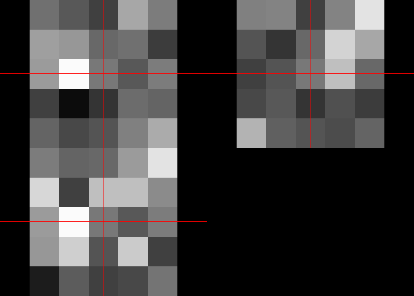

This section provides a brief introduction to viewing nifti files. Data are stored as rows, columns and slices. To view sagital image then assign a number to the row data.

#plot mca #sagittal
image(mca[50,,])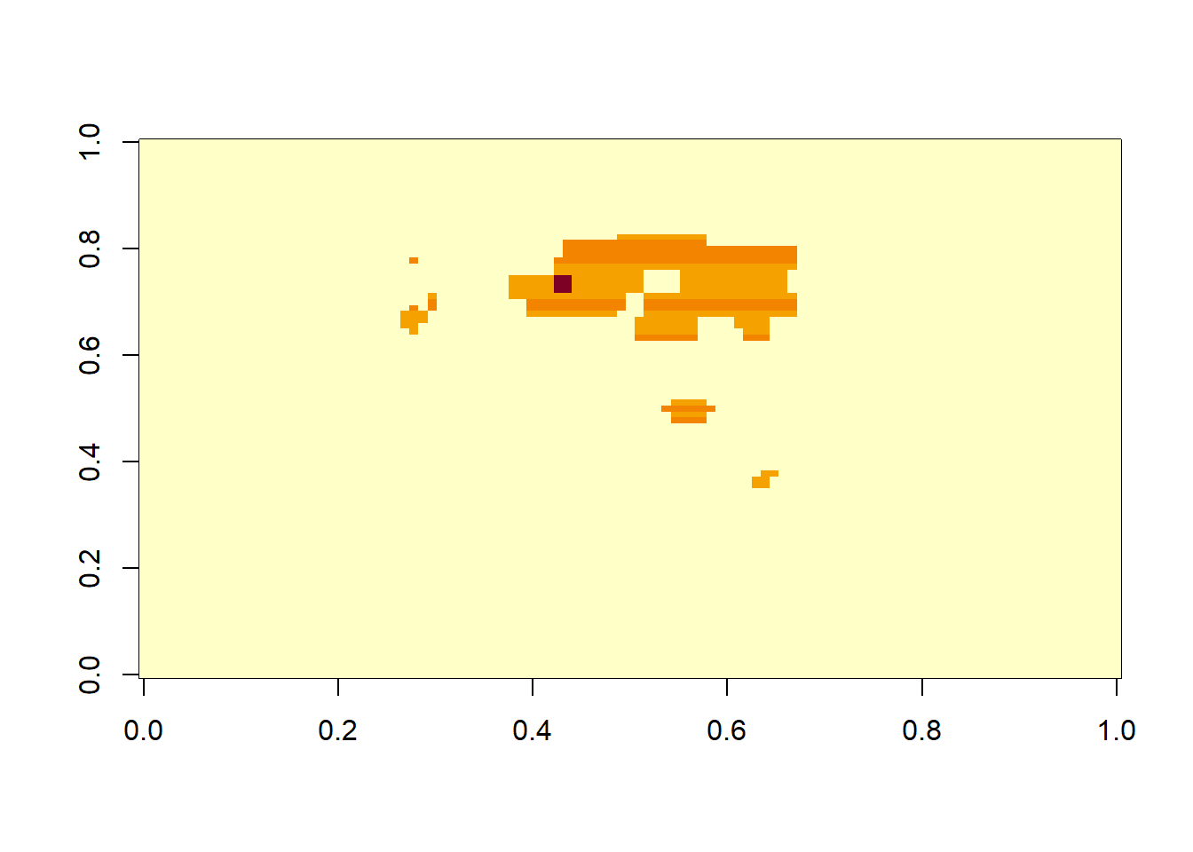 

To see coronal image, assign a number to the column data.

#plot mca #coronal
image(mca[,70,])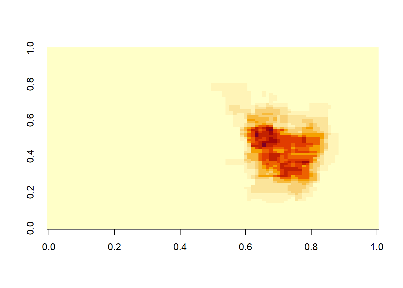 

To see axial image, assign a number to the slice data.

#plot mca #axial in third column
image(mca[,,35])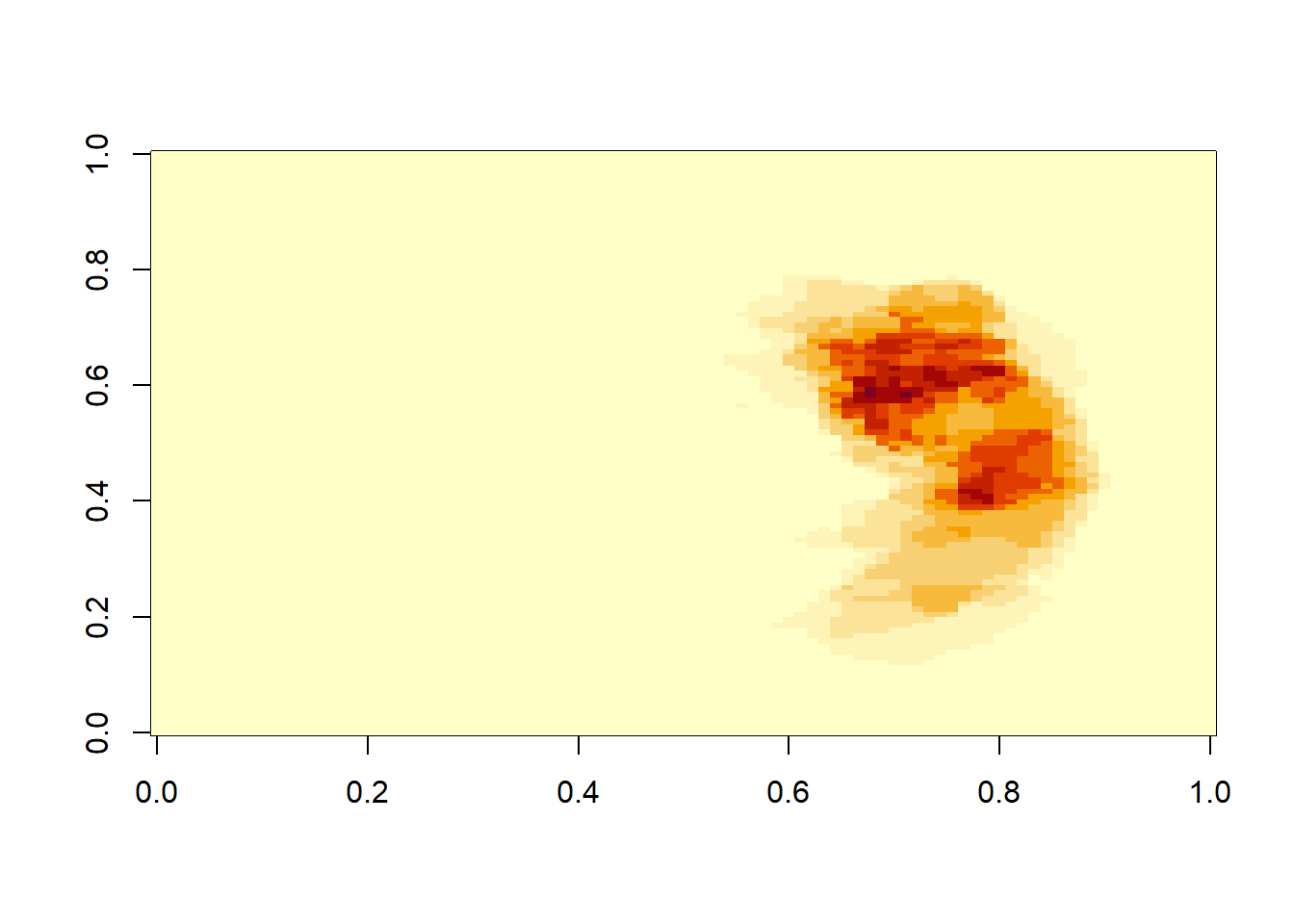 

3.0.2 Manipulating array of medical images

These arrays of medical images should be treated no differently from any other arrays. The imaging data are stored as arrays within the .Data slot in nifti.

Data can be subset using the square bracket. The image is referred to x (right to left), y (front to back), z (superior to inferior).

library(oro.nifti)
#extract data as array using @ function
img<-readNIfTI("./Data-Use/mca_notpa.nii.gz", reorient = FALSE) 
k<-img@.Data

#change x orientation to right to left 91*109*91
k1<-k[91:1,,] 
#access slice 35 to verify that the image orientation has been switched.
image(k1[,,35])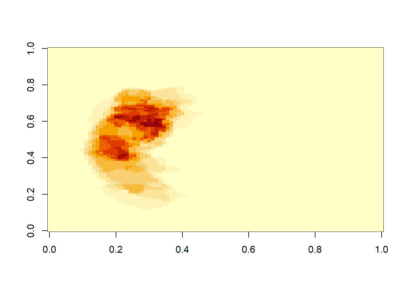

With the image now flipped to the other side, we can create an image by returning the array into its data slot.

img2<-img
img2@.Data <- k1
img2

NIfTI-1 format
  Type            : nifti
  Data Type       : 16 (FLOAT32)
  Bits per Pixel  : 32
  Slice Code      : 0 (Unknown)
  Intent Code     : 0 (None)
  Qform Code      : 0 (Unknown)
  Sform Code      : 1 (Scanner_Anat)
  Dimension       : 91 x 109 x 91
  Pixel Dimension : 2 x 2 x 2
  Voxel Units     : mm
  Time Units      : sec

Arrays can be manipulated to split an image into 2 separate images. Below is a function to split B0 and B1000 images from diffusion series.

#split dwi file into b0 and b1000
#assume that b1000 is the second volume
#dwi<-readNIfTI("....nii.gz",reorient = F)

DWIsplit<-function(D) {
  DWI<-readNIfTI(D,reorient = F)
  b1000<-dwi #dim (b1000) [1] 384 384  32   2
  k<-dwi@.Data
  b1000k<-k[,,,2] #dim(b1000k) [1] 384 384  32
  writeNIfTI(b1000k,"b1000")
}

Measurement of volume requires information on the dimensions of voxel.

#measure volume
A="./Ext-Data/3000F_mca_blur.nii"

VoxelDim<-function(A){
  library(oro.nifti)
  img<-readNIfTI(A,reorient = F)
  VoxDim<-pixdim(img)
Volume<-sum(img>.5)*VoxDim[2]*VoxDim[3]*VoxDim[4]/1000
Volume
}

VoxelDim(A)

Malformed NIfTI - not reading NIfTI extension, use at own risk!

[1] 69

Find unsigned angle between 2 vectors k and k1

Morpho::angle.calc(k,k1)

[1] 1.570771

Determine centre of gravity of an object.

#centre of gravity
neurobase::cog(img)

    dim1     dim2     dim3 
65.74983 53.09204 46.67048 

3.0.3 Combining arrays

This is an illustration of combining array using cbind.

#stack arrays
k2<-cbind(k,k1)
dim(k2) ### [1] 902629      2

[1] 902629      2

The abind function produces a different array output. Later we will repeat the same exercise using list function.

#combine multi-dimensional arrays 
ab<-abind::abind(k,k1)
dim(ab) ### [1]  91 109 182

[1]  91 109 182

This example uses 25 files. Rather than open one file at a time create a list from pattern matching.

library(oro.nifti)
library(abind)
library(CHNOSZ) # for working with arrays

CHNOSZ version 2.0.0 (2023-03-13)

reset: creating "thermo" object

OBIGT: loading default database with 1904 aqueous, 3448 total species

Attaching package: 'CHNOSZ'

The following object is masked from 'package:oro.nifti':

    slice

library(RNiftyReg)

Attaching package: 'RNiftyReg'

The following objects are masked from 'package:oro.nifti':

    pixdim, pixdim<-

#create a list using pattern matching
mca.list<-list.files(path="./Ext-Data/",pattern = "*.nii", full.names = TRUE)

#length of list
length(mca.list)

[1] 42

#read multiple files using lapply function

#use lappy to read in the nifti files
#note lapply returns a list
mca.list.nii <- lapply(mca.list, readNIfTI)

Malformed NIfTI - not reading NIfTI extension, use at own risk!

Malformed NIfTI - not reading NIfTI extension, use at own risk!
Malformed NIfTI - not reading NIfTI extension, use at own risk!
Malformed NIfTI - not reading NIfTI extension, use at own risk!
Malformed NIfTI - not reading NIfTI extension, use at own risk!
Malformed NIfTI - not reading NIfTI extension, use at own risk!
Malformed NIfTI - not reading NIfTI extension, use at own risk!
Malformed NIfTI - not reading NIfTI extension, use at own risk!
Malformed NIfTI - not reading NIfTI extension, use at own risk!
Malformed NIfTI - not reading NIfTI extension, use at own risk!
Malformed NIfTI - not reading NIfTI extension, use at own risk!
Malformed NIfTI - not reading NIfTI extension, use at own risk!
Malformed NIfTI - not reading NIfTI extension, use at own risk!
Malformed NIfTI - not reading NIfTI extension, use at own risk!
Malformed NIfTI - not reading NIfTI extension, use at own risk!
Malformed NIfTI - not reading NIfTI extension, use at own risk!
Malformed NIfTI - not reading NIfTI extension, use at own risk!
Malformed NIfTI - not reading NIfTI extension, use at own risk!
Malformed NIfTI - not reading NIfTI extension, use at own risk!
Malformed NIfTI - not reading NIfTI extension, use at own risk!
Malformed NIfTI - not reading NIfTI extension, use at own risk!
Malformed NIfTI - not reading NIfTI extension, use at own risk!
Malformed NIfTI - not reading NIfTI extension, use at own risk!
Malformed NIfTI - not reading NIfTI extension, use at own risk!
Malformed NIfTI - not reading NIfTI extension, use at own risk!

class(mca.list.nii)

[1] "list"

This example illustrates how to view the first image in the list.

#view each image in the list
neurobase::ortho2(mca.list.nii[[1]])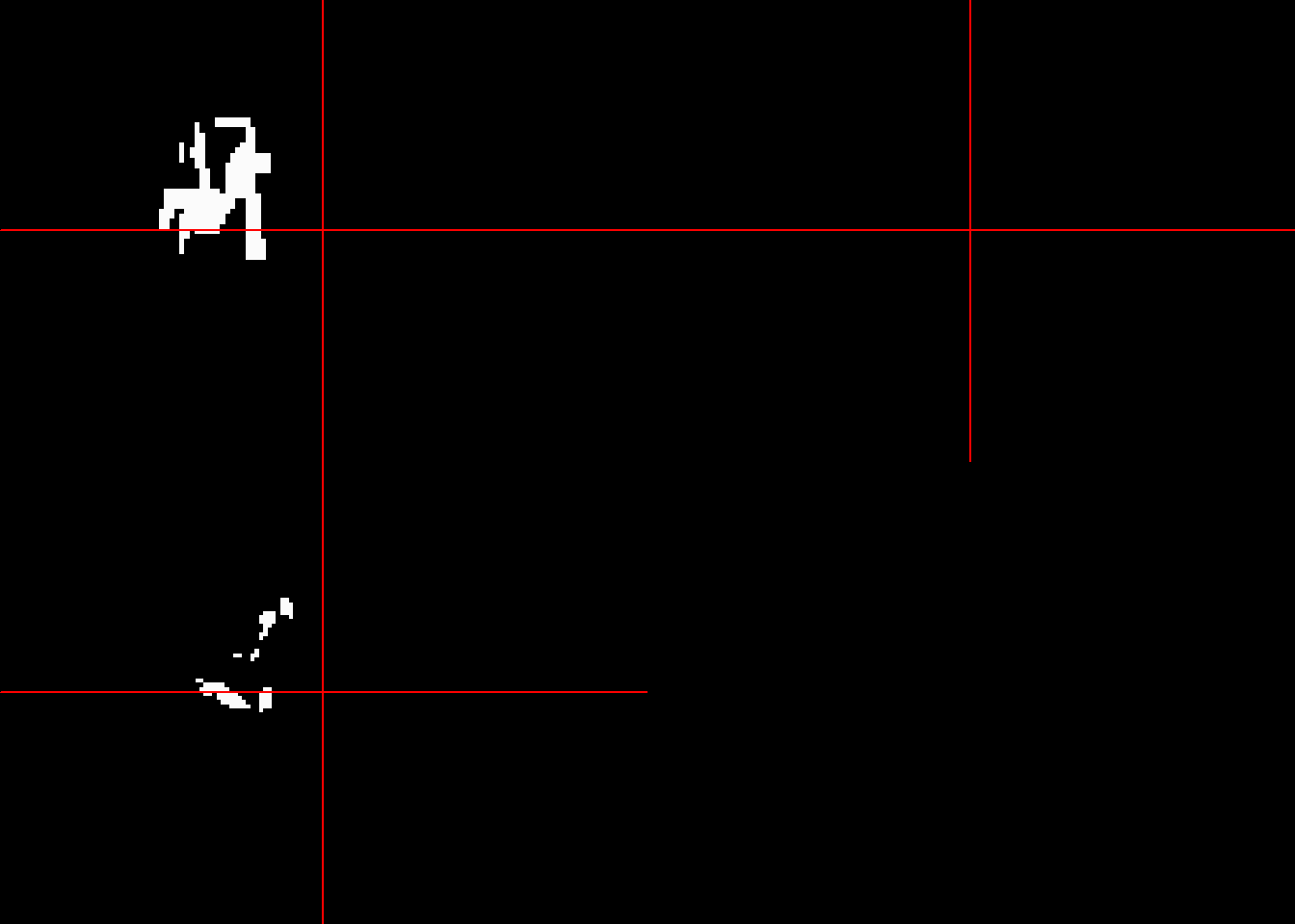

In this example, the first 3 segmented images from the list are averaged and viewed.

#view average image
mca_ave3<-(mca.list.nii[[5]]+mca.list.nii[[6]]+mca.list.nii[[7]])/3
neurobase::ortho2(mca_ave3)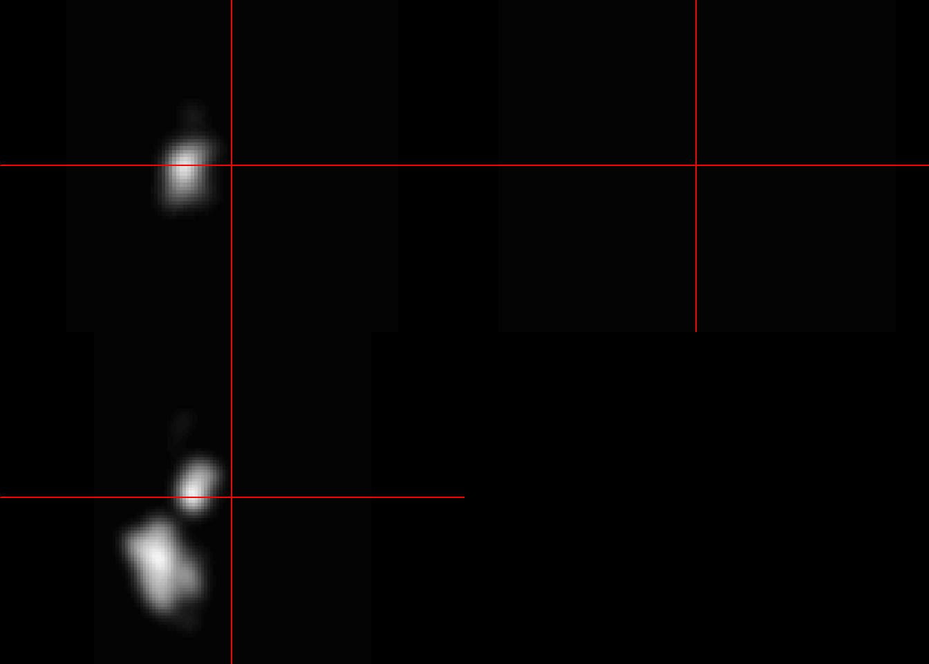

The output below is the same as above but is performed on arrays. The image_data function from oro.nifti library extracts the image attribute from the slot .Data.

#extract multiple arrays using lapply
mca.list.array<-lapply(mca.list.nii, img_data)

m3<-(mca.list.array[[5]]+mca.list.array[[6]]+mca.list.array[[7]])/3

#compare this with the output from above
neurobase::double_ortho(m3, mca_ave3)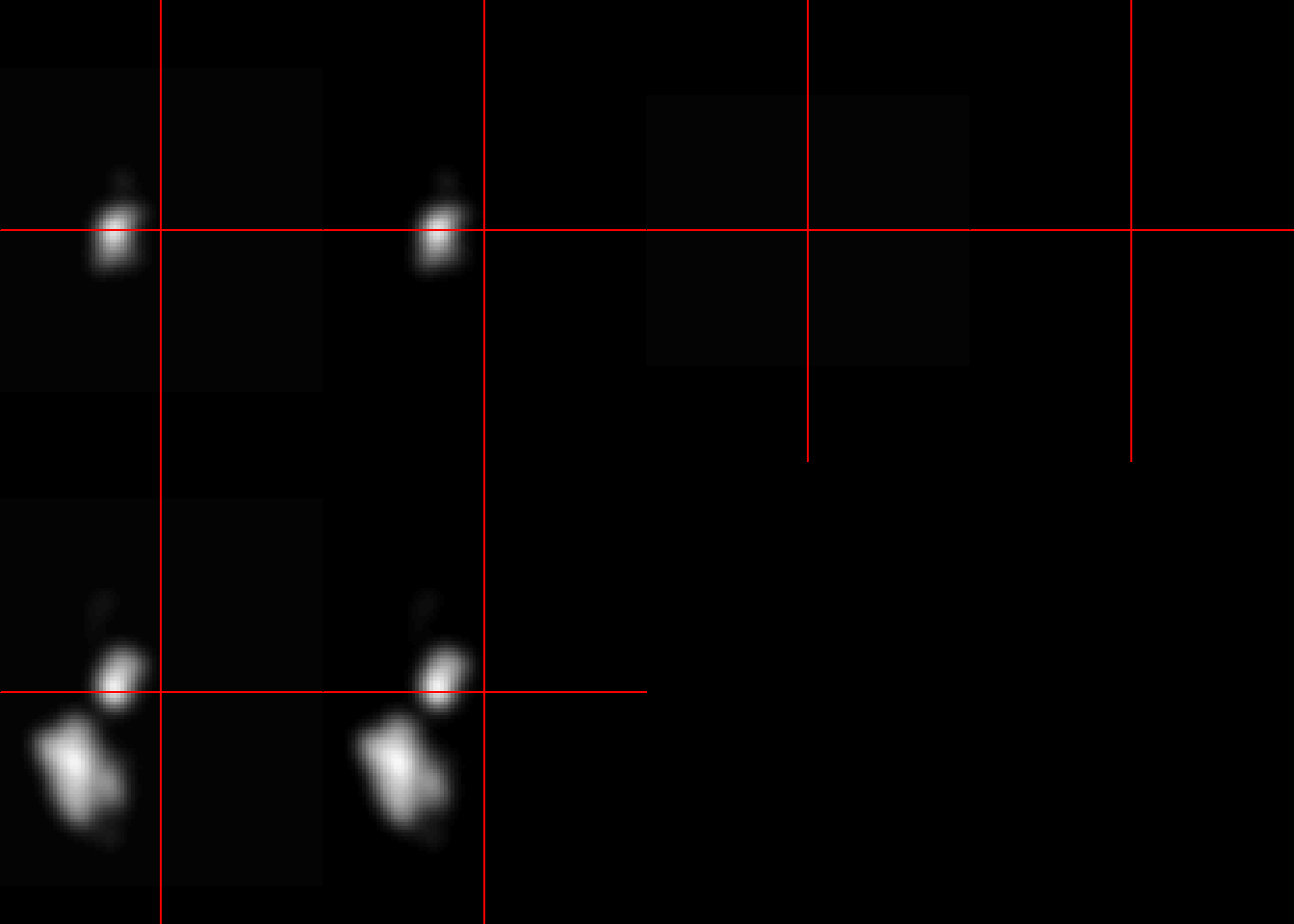

Arrays can be extracted from list using list2array function.

class(mca.list.array)

[1] "list"

#convert list to array
#CHNOSZ function
m.listarray<-CHNOSZ::list2array(mca.list.array)#91 109  91  25

class(m.listarray)

[1] "array"

3.0.4 Math operation on multidimensional array

Before illustrating more complex operations on ultidimensional array or tensor, let’s consider the basics of multidimensional array. The rank of a tensor represents the dimension of an array. Rank 0 represents 1 dimension and so on.

Here we use apply function to average over every element of the multidimensional array. The first argument of apply is the array, the second argument is the margin or the component for analysis and the last argument is the function. If the idea is to analyse the row then the margin argument is c(1), column then the margin argumen is c(2) and so on.

ma<-apply(m.listarray,c(1,2,3), mean)
neurobase::ortho2(ma)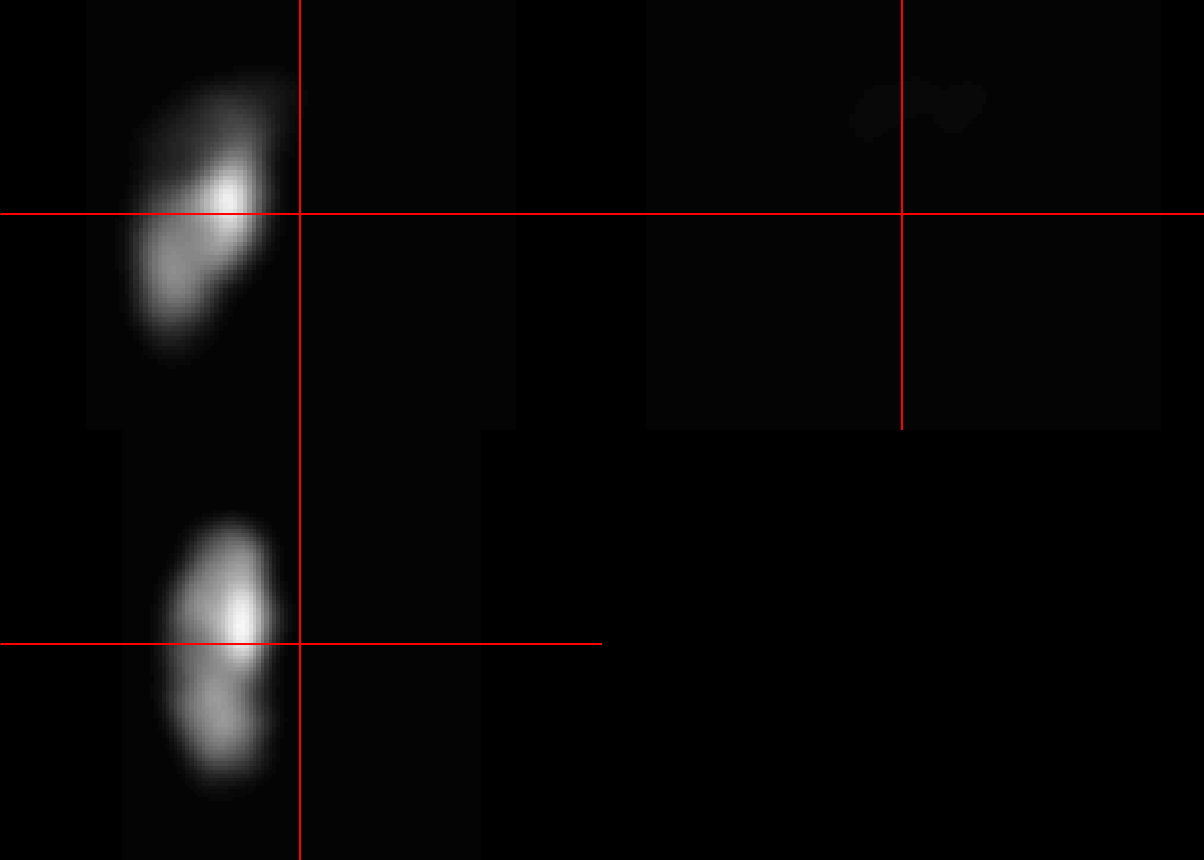

Thresholding can be performed using mask_img function. This function can also be used to create a mask.

ma_mask=neurobase::mask_img(ma, ma>0.1)

neurobase::double_ortho(ma_mask, ma)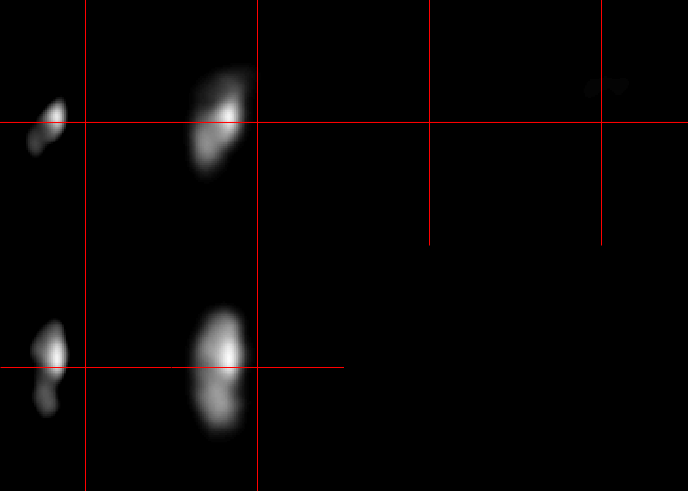

3.0.5 Math operation on list

In this example we us lapply to a function within a list. This is an example of a functional or a function which takes a function as an input and return a vector as an output. In this example, a functional operates on one element of the list at a time. This example of functional is the same as the function VoxelDim describes above.

vox=unlist(lapply(mca.list.nii, 
           function(A) sum(A>.5)*
             #obtain voxel dimensions
             oro.nifti::pixdim(A)[2]*
             oro.nifti::pixdim(A)[3]*
             oro.nifti::pixdim(A)[4]/1000
           ))

vox

 [1]   0.000   0.000   0.000   0.000  69.000   3.624   8.768  58.200 326.760
[10]   1.608   0.000   3.904   3.328  66.776 106.976  70.928  26.912  11.768
[19]  17.592  14.720 151.872  87.528   0.000  24.192  80.248 152.792  69.552
[28]  25.576   0.000   8.644   4.230   3.781   3.643   5.720   5.061   8.644
[37]   4.230   3.781   3.643   5.720   5.061  43.968

3.0.6 Vectorising nifti object

One way of handling imaging data for analysis is to flatten the image, then create an empty array of the same size to return the image.

#flatten 3D
niivector = as.vector(img[,,]) #902629

#Create empty array of same size to fill up
niinew = array(0, dim=dim(img))

#return to 3D
niinew = array(niivector, dim=dim(img))

#confirm
neurobase::ortho2(niinew)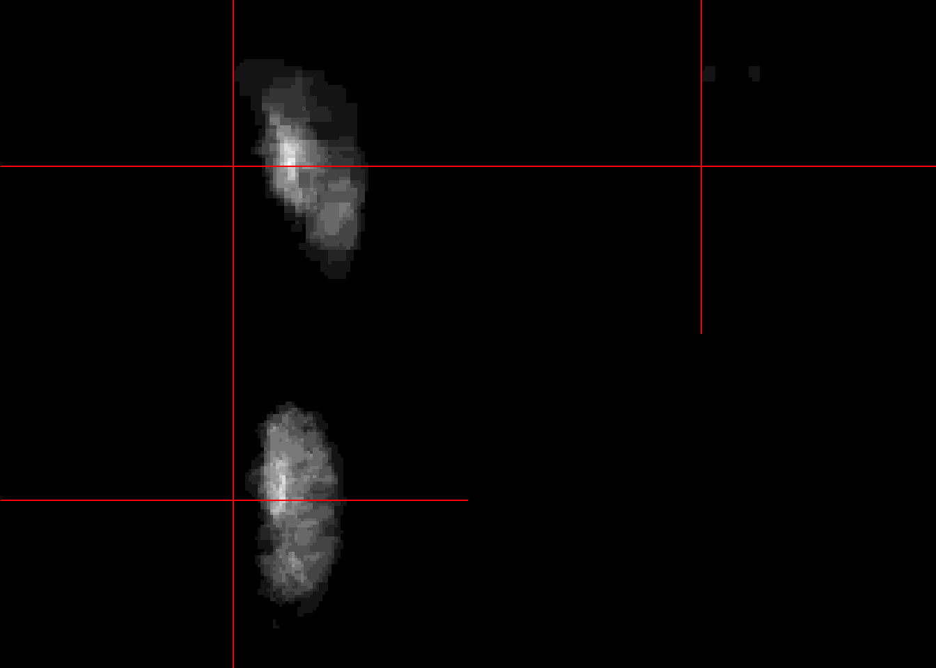

Another way of creating vector from the image is to use c function.

#vector can also be created using c
niivector2 = c(img[,,]) #902629

3.0.7 tar file

Image files can be large and are often stored as tar files. The tar (tgz file), untar, zip (gz file) and unzip function are from the utils library.

colin_1mm<-untar("./Data-Use/colin_1mm.tgz")
colinIm<-readNIfTI("colin_1mm") #1 x 1 x 1
class(colinIm)

[1] "nifti"
attr(,"package")
[1] "oro.nifti"

neurobase::ortho2(colinIm)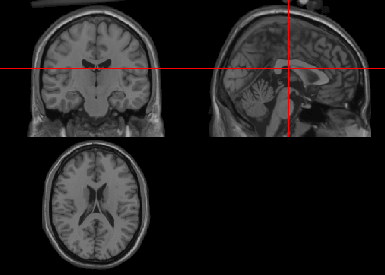

The readNIfTI call can open gz file without the need to call unzip function.

library(RNiftyReg)
epi_t2<- readNIfTI(system.file("extdata", "epi_t2.nii.gz", package="RNiftyReg"))
class(epi_t2)

[1] "nifti"
attr(,"package")
[1] "oro.nifti"

neurobase::ortho2(epi_t2)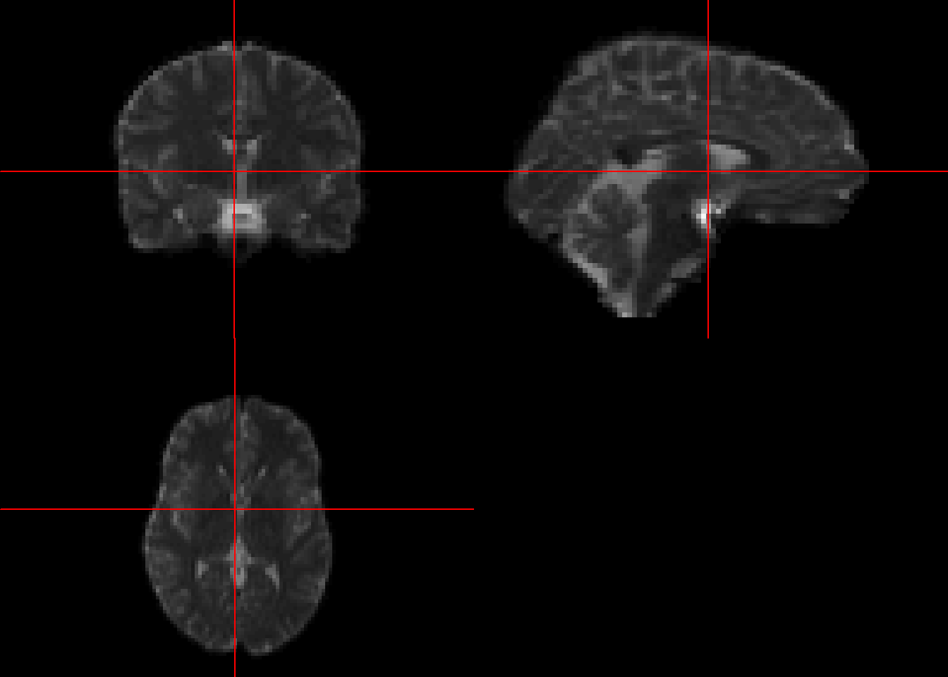

3.0.8 Image registration

There are many different libraries for performing registration.

library(RNiftyReg)

#example from data
source<-readNifti("./Data-Use/mca10_pca10_border10.nii.gz")
pixdim(source)

[1] 2 2 2

colin_1mm<-untar("./Data-Use/colin_1mm.tgz")
target<-readNifti("colin_1mm")
pixdim(target)

[1] 1 1 1 1

target

Image array of mode "double" (54.2 Mb)
- 181 x 217 x 181 x 1 voxels
- 1 x 1 x 1 mm x 1 s per voxel

#register source to target 
result <- niftyreg(source, target)
#affine transformation
result$forwardTransforms

[[1]]
NiftyReg affine matrix:
    0.773388    0.569432    0.471194    4.534728
   -0.595046    0.720880   -0.807965  -19.901979
   -0.562192   -0.069332    0.552411   21.512533
    0.000000    0.000000    0.000000    1.000000

#image in target space
result$image

Image array of mode "double" (54.2 Mb)
- 181 x 217 x 181 voxels
- 1 x 1 x 1 mm per voxel

neurobase::ortho2(result$image)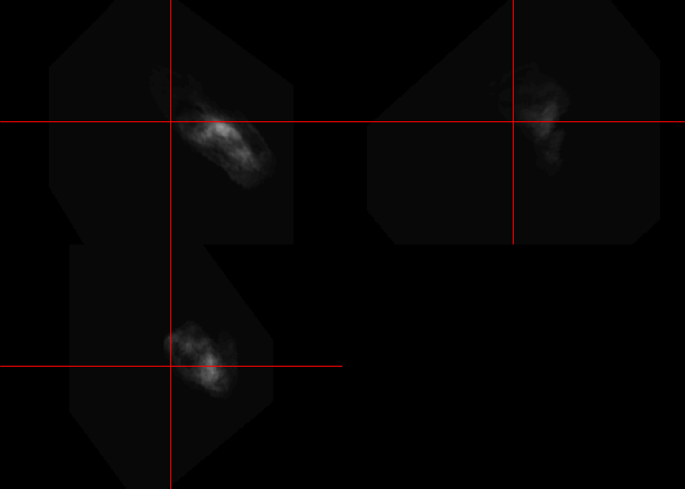

Output from RNiftyReg are niftiImage objects. They can be converted to oro.nifti objects using nii2oro function.

otarget<-nii2oro(target)
oimage<-nii2oro(result$image)

overlay(otarget, y=oimage,z = 90, plot.type = "single" )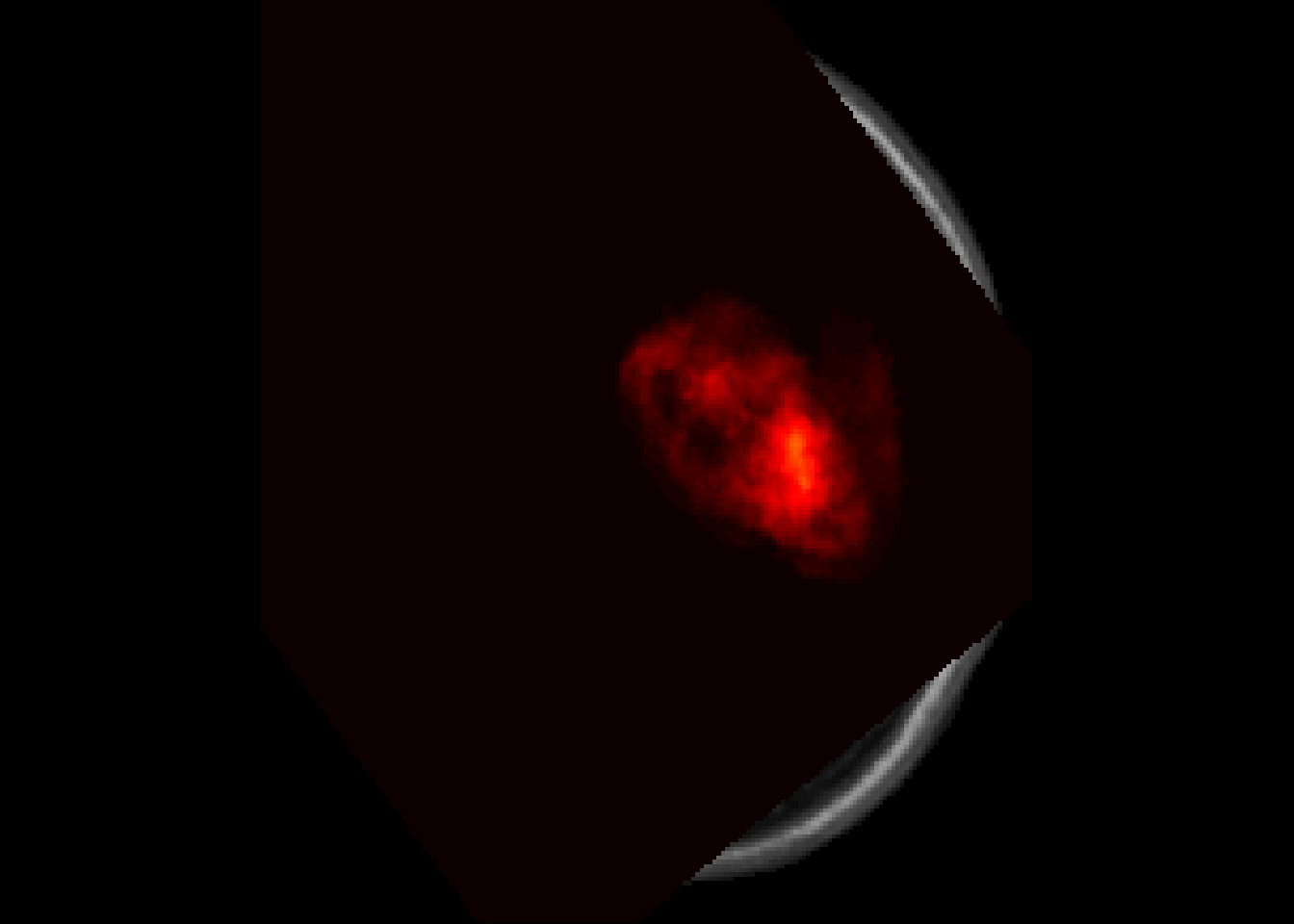

3.0.9 Rescaling

Perform affine registration and resampling of image using the transformation file.

#affine
ica1000<-readNifti("./Ext-Data/1000M_ica.nii")
ica1000

Image array of mode "double" (6.9 Mb)
- 91 x 109 x 91 voxels
- 2 x 2 x 2 mm per voxel

colin_affine<-buildAffine(source=ica1000, target=target)
#apply transformation from above
#assume 1000M_ica.nii and source are in the same space
colin_like<-applyTransform(colin_affine,ica1000)
neurobase::ortho2(colin_like)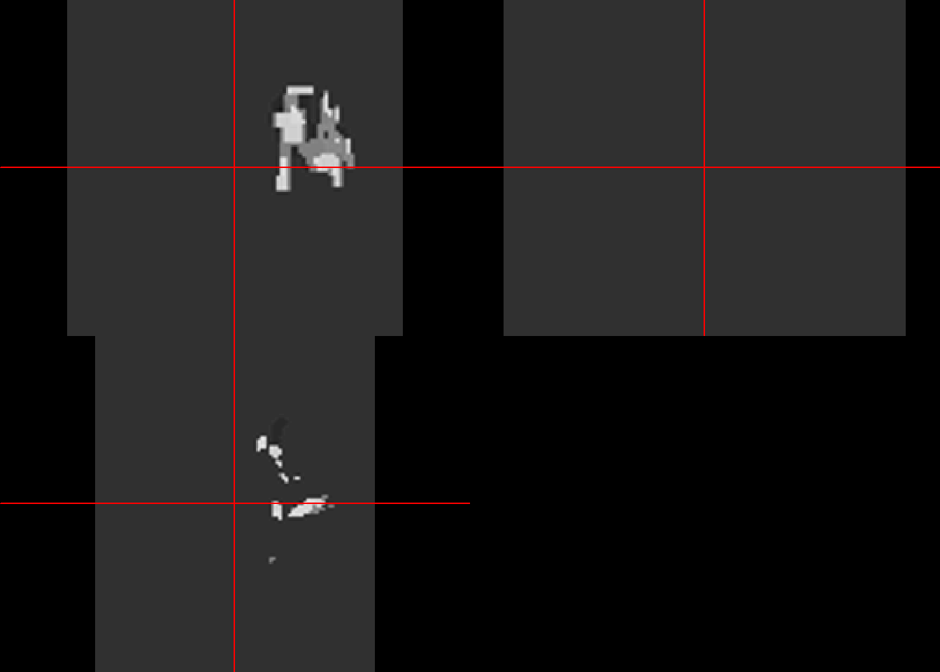

Resampling an image to different dimensions. This example is different from above in which rescaling is performed as part of registration to higher resolution image. Here the rescale function from RNiftyReg library is used to change the dimensions from 1x1x1 mm to 2x2x2 mm.

ica1000.rescale<-RNiftyReg::rescale(ica1000,c(.5,.5,.5))

ica1000

Image array of mode "double" (6.9 Mb)
- 91 x 109 x 91 voxels
- 2 x 2 x 2 mm per voxel

#compare with rescale

ica1000.rescale

Image array of mode "double" (855.6 Kb)
- 45 x 54 x 45 voxels
- 4 x 4 x 4 mm per voxel

3.0.10 MNI template

There are several different MRI templates. The well known one is the MNI 152 template (Mazziotta J 2001). This was developed from male right-handed medical students. The MNI 152 is also known as International Consortium for Brain Mapping (ICBM) 152.

The Colin high resolution template was obtained by scanning the same individual 27 times (Holmes CJ 1998). This template was registered to the MNI 305 template and has been used as target template by some investigators.

3.0.11 Atlases

A list of available atlases for human and animals is available at https://loni.usc.edu/research/atlases.

3.0.11.1 AAL atlas

The automated anatomical labeling (AAL) atlas of activation contains 45 volume of interest in each hemisphere (Tzourio-Mazoyer N 2002). The atlas is aligned to MNI 152 coordinates. The updated AAL has additional parcellation of orbitofrontal cortex. AAL3 update includes further parcellation of thalamus.

library(rgl)
library(misc3d)
library(MNITemplate)
#source("https://neuroconductor.org/neurocLite.R")
#neuro_install('aal')
library(aal)
library(neurobase)
library(magick)

Linking to ImageMagick 6.9.12.3
Enabled features: cairo, freetype, fftw, ghostscript, heic, lcms, pango, raw, rsvg, webp
Disabled features: fontconfig, x11

library(oro.nifti)

img = aal_image()
template = readMNI(res = "2mm")
cut <- 4500
dtemp <- dim(template)

# All of the sections you can label
labs = aal_get_labels()

# highlight - in this case the Cingulate_Post_L
cingulate = labs$index[grep("Cingulate_Post_R", labs$name)]

#mask of object for rendering
mask = remake_img(vec = img %in% cingulate, img = img)

#contour for MNI template
contour3d(template, x=1:dtemp[1], y=1:dtemp[2], z=1:dtemp[3], level = cut, alpha = 0.1, draw = TRUE)

#contour for mask
contour3d(mask, level = c(0.5), alpha = c(0.5), add = TRUE, color=c("red") )

### add text
text3d(x=dtemp[1]/2, y=dtemp[2]/2, z = dtemp[3]*0.98, text="Top")
text3d(x=-0.98, y=dtemp[2]/2, z = dtemp[3]/2, text="Right")

#create movie
#movie file is saved to temporary folder
#movie3d(spin3d(),duration=30)

#add digital map of mca territory
MCA<-readNIfTI("./Data-Use/MCA_average28_MAP_100.nii")

Malformed NIfTI - not reading NIfTI extension, use at own risk!

#mask2 = remake_img(vec = img %in% source, img = img)
contour3d(template, x=1:dtemp[1], y=1:dtemp[2], z=1:dtemp[3], level = cut, alpha = 0.1, draw = TRUE)

#contour for mask
contour3d(MCA, level = c(0.5), alpha = c(0.5), add = TRUE, color=c("Yellow"))
#add frontal
angular = labs$index[grep("Angular_R", labs$name)]
#mask of object for rendering
mask2 = remake_img(vec = img %in% angular, img = img)
contour3d(mask2, level = c(0.5), alpha = c(0.5), add = TRUE, color=c("red"))
#add cingulate
contour3d(mask, level = c(0.5), alpha = c(0.5), add = TRUE, color=c("blue"))
### add text
text3d(x=dtemp[1]/2, y=dtemp[2]/2, z = dtemp[3]*0.98, text="Top")
text3d(x=-0.98, y=dtemp[2]/2, z = dtemp[3]/2, text="Right")

3.0.11.2 Eve template

The Eve template is from John Hopkins (“Atlas-Based Whole Brain White Matter Analysis Using Large Deformation Diffeomorphic Metric Mapping: Application to Normal Elderly and Alzheimer’s Disease Participants.” 2009). It is a single subject high resolution white matter atlas that has been morphed into MNI 152 coordinates. The atlas is parcellated into 176 regions based on ICBM-DTI-81 atlas.

#source("https://neuroconductor.org/neurocLite.R")
#neuro_install('EveTemplate', release = "stable", release_repo = "github")

library(EveTemplate)

eve_labels = readEveMap(type = "II")
eve_labels

NIfTI-1 format
  Type            : nifti
  Data Type       : 4 (INT16)
  Bits per Pixel  : 16
  Slice Code      : 0 (Unknown)
  Intent Code     : 0 (None)
  Qform Code      : 2 (Aligned_Anat)
  Sform Code      : 1 (Scanner_Anat)
  Dimension       : 181 x 217 x 181
  Pixel Dimension : 1 x 1 x 1
  Voxel Units     : mm
  Time Units      : Unknown

neurobase::ortho2(eve_labels)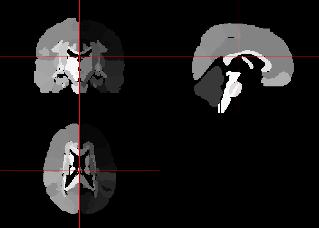

library(RColorBrewer)
library(tidyverse)

── Attaching core tidyverse packages ──────────────────────── tidyverse 2.0.0 ──
✔ dplyr     1.1.2     ✔ readr     2.1.4
✔ forcats   1.0.0     ✔ stringr   1.5.0
✔ ggplot2   3.5.1     ✔ tibble    3.2.1
✔ lubridate 1.9.2     ✔ tidyr     1.3.0
✔ purrr     1.0.1     
── Conflicts ────────────────────────────────────────── tidyverse_conflicts() ──
✖ dplyr::filter() masks stats::filter()
✖ dplyr::lag()    masks stats::lag()
✖ dplyr::slice()  masks CHNOSZ::slice(), oro.nifti::slice()
ℹ Use the conflicted package (<http://conflicted.r-lib.org/>) to force all conflicts to become errors

unique_labs = eve_labels %>% 
  c %>% 
  unique %>% 
  sort 
breaks = unique_labs
rf <- colorRampPalette(rev(brewer.pal(11,'Spectral')))
cols <- rf(length(unique_labs))

neurobase::ortho2(eve_labels, col = cols, breaks = c(-1, breaks))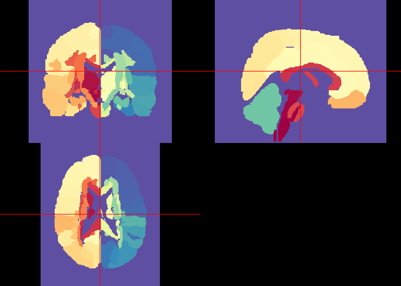

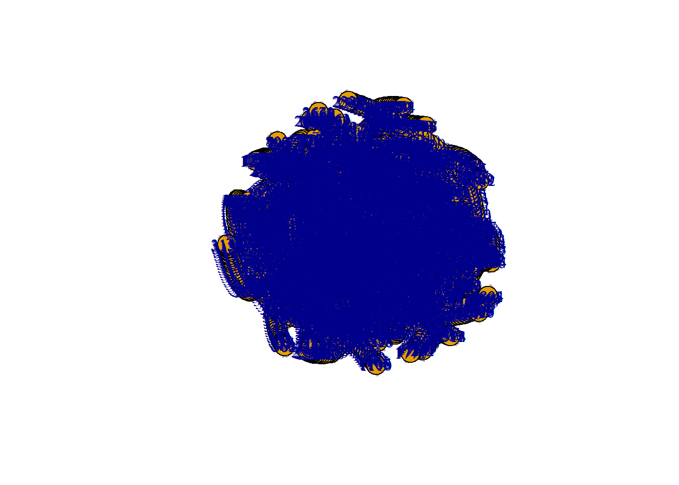
3.0.11.3 Sensorimotor tract atlas

Template for corticofugal tracts from primary motor cortex, dorsal premotor cortex, ventral premotor cortex, supplementary motor area (SMA), pre-supplementary motor area (preSMA), and primary somatosensory cortex is available from (Derek B Archer 2018). Below is an illustration of the M1 tract obtained from LRNLAB.

RightM1<-readNifti("./Ext-Data/Right-M1-S-MATT.nii")

neurobase::ortho2(RightM1)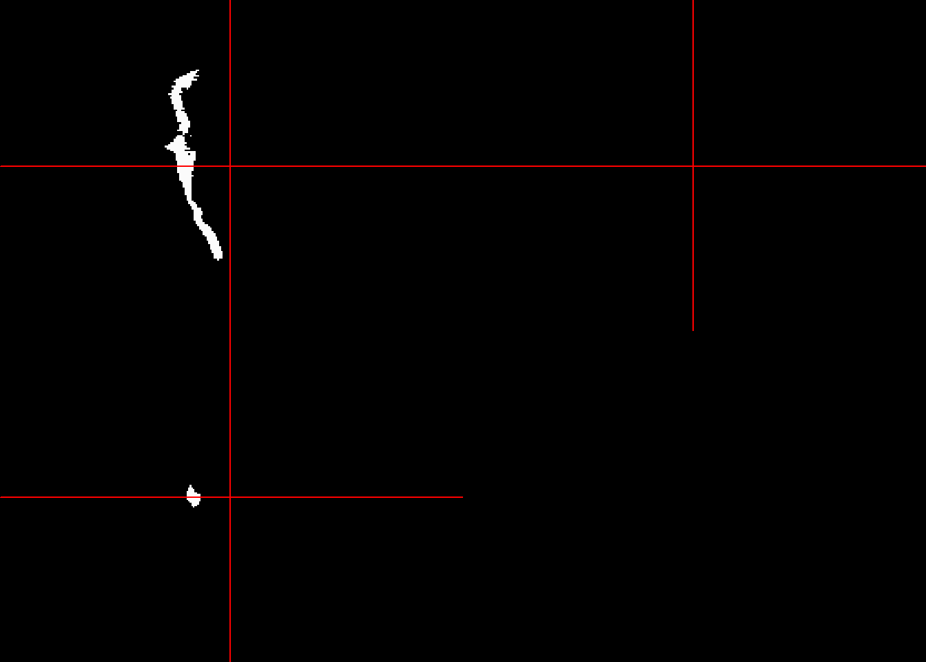

#to down weight the voxel from 1 mm to 2 mm
RightM1.rescale<-RNiftyReg::rescale(RightM1,c(.5,.5,.5))

RightM1o<-nii2oro(RightM1)

#dimensions of RightM1o (182 218 182) and eve_labels (181 217 181) are dissimilar
#overlay(eve_labels, y=RightM1o, z=90,plot.type="single")

3.1 Neurons and arteries

The swc format is used for examining morphology of neurons (K. Mehta and Ascoli 2023) or arteries (Decroocq et al. 2023). The file represent neurons or arteries as connected components. Example is provided from the nat library.

3.1.1 Neurons

library(nat)

Registered S3 method overwritten by 'nat':
  method             from
  as.mesh3d.ashape3d rgl 

Some nat functions depend on a CMTK installation. See ?cmtk and README.md for details.

Attaching package: 'nat'

The following objects are masked from 'package:lubridate':

    intersect, setdiff, union

The following objects are masked from 'package:dplyr':

    intersect, setdiff, union

The following object is masked from 'package:RNiftyReg':

    xform

The following object is masked from 'package:oro.nifti':

    origin

The following objects are masked from 'package:base':

    intersect, setdiff, union

n = Cell07PNs[[1]]
# inspect its internal structure
str(n)

List of 24
 $ CellType     : chr "DA1"
 $ NeuronName   : chr "EBH11R"
 $ InputFileName: 'AsIs' chr "/GD/projects/PN2/TransformedTraces/DA1/EBH11R.tasc"
 $ CreatedAt    : POSIXt[1:1], format: "2006-01-18 02:21:14"
 $ NodeName     : Named chr "jefferis.joh.cam.ac.uk"
  ..- attr(*, "names")= chr "nodename"
 $ InputFileStat:'data.frame':  1 obs. of  10 variables:
  ..$ size  : num 15379
  ..$ isdir : logi FALSE
  ..$ mode  : 'octmode' int 644
  ..$ mtime : POSIXt[1:1], format: "2006-01-12 11:52:01"
  ..$ ctime : POSIXt[1:1], format: "2006-01-12 11:52:01"
  ..$ atime : POSIXt[1:1], format: "2006-01-18 02:21:14"
  ..$ uid   : int 501
  ..$ gid   : int 501
  ..$ uname : chr "jefferis"
  ..$ grname: chr "jefferis"
 $ InputFileMD5 : Named chr "fcacee3f874cbe2c6ad96214e6fee337"
  ..- attr(*, "names")= 'AsIs' chr "/GD/projects/PN2/TransformedTraces/DA1/EBH11R.tasc"
 $ NumPoints    : int 180
 $ StartPoint   : num 1
 $ BranchPoints : num [1:16] 34 48 51 75 78 95 98 99 108 109 ...
 $ EndPoints    : num [1:18] 1 42 59 62 80 85 96 100 102 112 ...
 $ NumSegs      : int 33
 $ SegList      :List of 33
  ..$ : int [1:34] 1 2 3 4 5 6 7 8 9 10 ...
  ..$ : int [1:9] 34 35 36 37 38 39 40 41 42
  ..$ : num [1:7] 34 43 44 45 46 47 48
  ..$ : int [1:4] 48 49 50 51
  ..$ : int [1:9] 51 52 53 54 55 56 57 58 59
  ..$ : num [1:4] 51 60 61 62
  ..$ : num [1:14] 48 63 64 65 66 67 68 69 70 71 ...
  ..$ : int [1:4] 75 76 77 78
  ..$ : int [1:3] 78 79 80
  ..$ : num [1:6] 78 81 82 83 84 85
  ..$ : num [1:11] 75 86 87 88 89 90 91 92 93 94 ...
  ..$ : int [1:2] 95 96
  ..$ : num [1:3] 95 97 98
  ..$ : int [1:2] 98 99
  ..$ : int [1:2] 99 100
  ..$ : num [1:3] 99 101 102
  ..$ : num [1:7] 98 103 104 105 106 107 108
  ..$ : int [1:2] 108 109
  ..$ : int [1:4] 109 110 111 112
  ..$ : num [1:4] 109 113 114 115
  ..$ : int [1:3] 115 116 117
  ..$ : num [1:3] 115 118 119
  ..$ : int [1:3] 119 120 121
  ..$ : num [1:14] 119 122 123 124 125 126 127 128 129 130 ...
  ..$ : num [1:2] 108 135
  ..$ : int [1:9] 135 136 137 138 139 140 141 142 143
  ..$ : int [1:6] 143 144 145 146 147 148
  ..$ : num [1:7] 143 149 150 151 152 153 154
  ..$ : num [1:7] 135 155 156 157 158 159 160
  ..$ : int [1:6] 160 161 162 163 164 165
  ..$ : num [1:5] 160 166 167 168 169
  ..$ : int [1:4] 169 170 171 172
  ..$ : num [1:9] 169 173 174 175 176 177 178 179 180
 $ d            :'data.frame':  180 obs. of  7 variables:
  ..$ PointNo: int [1:180] 1 2 3 4 5 6 7 8 9 10 ...
  ..$ Label  : num [1:180] 2 2 2 2 2 2 2 2 2 2 ...
  ..$ X      : num [1:180] 187 187 188 188 188 ...
  ..$ Y      : num [1:180] 133 131 130 129 129 ...
  ..$ Z      : num [1:180] 88.2 90.6 93.1 95 97.5 ...
  ..$ W      : num [1:180] 1.01 1.27 1.14 1.27 1.27 1.27 1.27 1.27 1.27 1.27 ...
  ..$ Parent : num [1:180] -1 1 2 3 4 5 6 7 8 9 ...
 $ OrientInfo   :List of 5
  ..$ AxonOriented: logi TRUE
  ..$ AVMPoint    : logi NA
  ..$ AVLPoint    : logi NA
  ..$ Scl         : num [1:3] 1 1 1
  ..$ NewAxes     : num [1:3] 1 2 3
 $ SegOrders    : num [1:33] 1 2 2 3 4 4 3 4 5 5 ...
 $ MBPoints     : int [1:2] 34 48
 $ LHBranchPoint: int 75
 $ SegTypes     : num [1:33] 1 3 1 3 3 3 1 2 2 2 ...
 $ AxonSegNos   :List of 3
  ..$ PreMBAxons : int 1
  ..$ MBAxons    : int 3
  ..$ PostMBAxons: int 7
 $ LHSegNos     : num [1:26] 8 9 10 11 12 13 14 15 16 17 ...
 $ MBSegNos     :List of 2
  ..$ : int 2
  ..$ : num [1:3] 4 5 6
 $ NumMBBranches: num 2
 $ AxonLHEP     : num 72
 - attr(*, "class")= chr [1:2] "neuron" "list"

# summary of 3D points
summary(xyzmatrix(n))

       X               Y                Z        
 Min.   :186.9   Min.   : 90.36   Min.   : 88.2  
 1st Qu.:225.6   1st Qu.: 97.56   1st Qu.:103.4  
 Median :258.4   Median :102.70   Median :112.9  
 Mean   :249.4   Mean   :104.03   Mean   :120.9  
 3rd Qu.:277.7   3rd Qu.:109.04   3rd Qu.:139.0  
 Max.   :289.5   Max.   :132.71   Max.   :157.3  

# identify 3d location of endpoints
xyzmatrix(n)[endpoints(n),]

           X         Y         Z
1   186.8660 132.70932  88.20393
42  224.7067 109.86362 153.58749
59  229.6343  92.30637 157.29700
62  226.8855  90.36325 147.59602
80  249.8864  93.59079 136.77795
85  253.0099  90.94904 137.34921
96  264.0801  98.53390 121.89463
100 266.3223  98.73241 116.46558
102 267.5460  98.59859 112.85608
112 271.0762 102.67288 100.84955
117 274.6128 100.92061 103.28772
121 277.3920 102.19148 102.69473
134 287.1214 101.43365 103.30740
148 281.7958  96.63987 101.08075
154 276.6551  95.09809  99.22113
165 278.3287 113.75627 104.87700
172 282.3069 111.93213 105.65492
180 289.5364 111.96014 109.18281

Plotting a neuron

plot(n)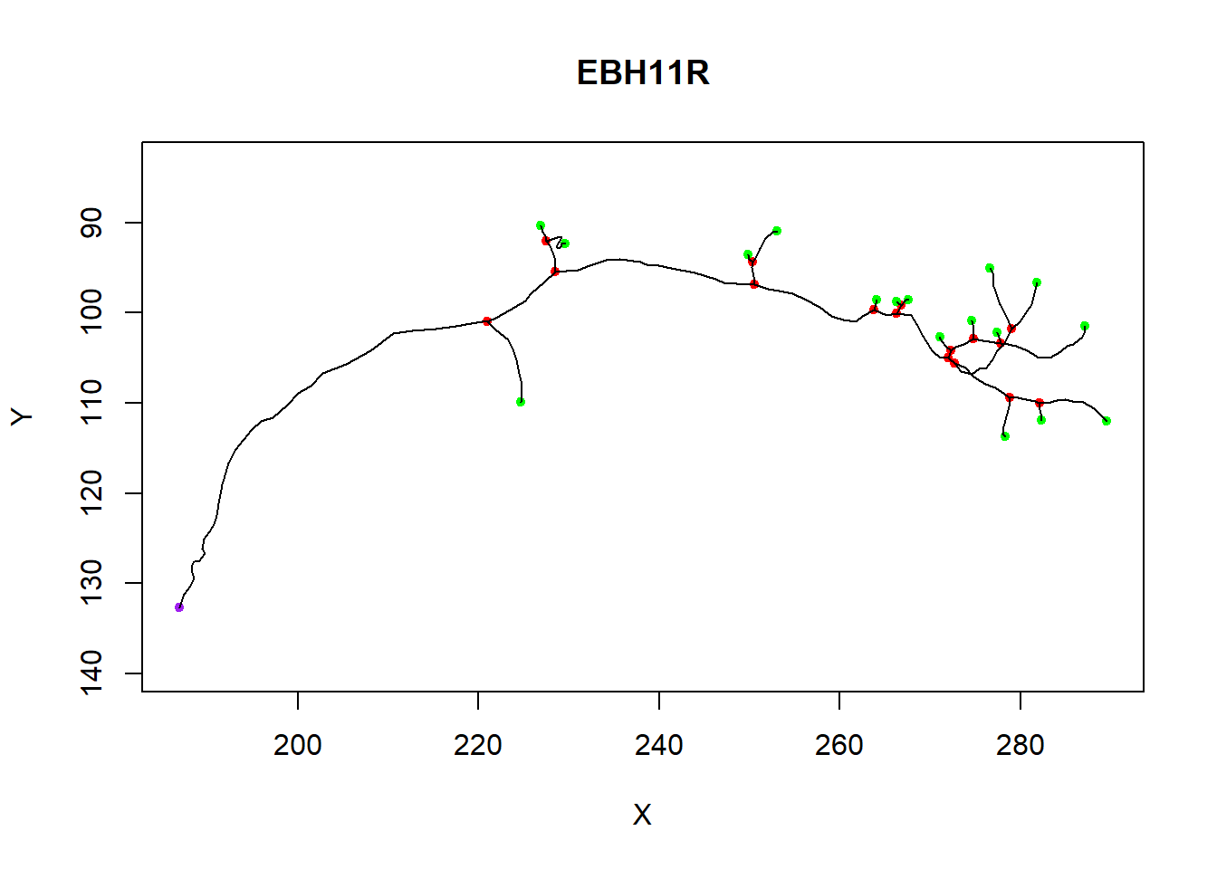

3.1.2 Arteries

The read.ngraph.swc function provides a link to the igraph library.

library(nat)
a<-read.ngraph.swc("./Ext-Data/swc_files/BG0002.CNG.swc")
plot(a)

“Atlas-Based Whole Brain White Matter Analysis Using Large Deformation Diffeomorphic Metric Mapping: Application to Normal Elderly and Alzheimer’s Disease Participants.” 2009. Neuroimage 46 (2): 486–99. https://doi.org/10.1016/j.neuroimage.2009.01.002.

Decroocq, Méghane, Carole Frindel, Pierre Rougé, Makoto Ohta, and Guillaume Lavoué. 2023. “Modeling and Hexahedral Meshing of Cerebral Arterial Networks from Centerlines.” Medical Image Analysis 89: 102912. https://doi.org/https://doi.org/10.1016/j.media.2023.102912.

Derek B Archer, Stephen A Coombes, David E Vaillancourt. 2018. “A Template and Probabilistic Atlas of the Human Sensorimotor Tracts Using Diffusion MRI.” Cerebral Cortex 28 (5): 1685--1699. https://doi.org/10.1093/cercor/bhx066.

Holmes CJ, Collins L, Hoge R. 1998. “Enhancement of MR Images Using Registration for Signal Averaging.” J Comput Assist Tomogr 22: 324–33. https://doi.org/10.1097/00004728-199803000-00032.

K. Mehta, J. Ogden, B. Ljungquist, and G. A. Ascoli. 2023. “Online Conversion of Reconstructed Neural Morphologies into Standardized SWC Format.” Nature Communications 14: 7429. https://doi.org/10.1038/s41467-023-42931-x.

Mazziotta J, Evans A, Toga A. 2001. “A Probabilistic Atlas and Reference System for the Human Brain: International Consortium for Brain Mapping (ICBM).” Philos Trans R Soc Lond B Biol Sci 356 (1412): 1293–1322. https://doi.org/10.1098/rstb.2001.0915.

Tzourio-Mazoyer N, Papathanassiou D, Landeau B. 2002. “Automated Anatomical Labeling of Activations in SPM Using a Macroscopic Anatomical Parcellation of the MNI MRI Single-Subject Brain.” Neuroimage 15 (1): 273–89. https://doi.org/10.1006/nimg.2001.0978.