library(DiagrammeR)

grViz("digraph flowchart {
      # node definitions with substituted label text
      node [fontname = Helvetica, shape = circle]
      tab1 [label = '@@1']
      tab2 [label = '@@2']

# edge definitions with the node IDs
      tab1 -> tab1
      tab1-> tab2
      tab2->tab1
      tab2->tab2;
}
      [1]: 'A'
      [2]: 'B'
")8 Bayesian Analysis
8.1 Bayesian belief
Bayes Theorem deals with the impact of information update on current belief expresses in terms of probability. \(P(A|B)\) is the posterior probability of A given knowledge of B. \(P(A)\) is the prior probability. \(P(B|A)\) is the conditional probability of B given A. \(P(A|B)=P(B|A) * P(A)/P(B)\)$
Bayes’ theorem can be expressed in terms of odds and post-test probabilities. This concept had been used in the analysis of the post-test probabilities of stroke related to the use of ABCD2. In this case the likelihood ratio and pretest probability of stroke in patients with TIA is used to calculate the post-test probability.
| Disease + | Disease - | |
|---|---|---|
| ABCD2>4 | TP | FP |
| ABCD2<5 | FN | TN |
\(PLR=\frac{P(ABCD2+|Stroke)}{P(ABCD2+|NoStroke)}\)
One can interpret the likelihood ratio in terms of Bayes theorem. To derive the post-test odds, the PLR is multiplied by the pre-test odds. The post-test odds is given by the product of the pre-test odds and the likelihood ratio.
\(Odds_{Post\ Test}=Odds_{Pre\ Test} * PLR\)
In turn, the post-test probabilities is calculated from the post-test odds.
\(Prob_{Post\ Test}=\frac{Odds_{Post\ Test}}{1+Odds_{Post\ Test}}\)
8.1.1 Conditional probability
Two events are independent if
Or
It follows that the events A and B occur simultaneously P(A∩B) is given by the probability of event A and probability of event B given that A has occurred.
If events A and B are independent then P(A∩B) is given by the probability of event A and probability of event B.
8.1.1.1 Bayes Rule
For a sample space (A) containing n different subspaces (A1, A2….An) and A is a subset of the larger sample space B+ and B-, the probability that A is a member of B+an be given by P(A|B+). This can be divised as a tree structure with one branch given by the product of P(B+) and P(A|B+) and the other P(B-) and P(A|B-). The probability of B is given by the sum of P(B+)P(A|B+) and P(B-)P(A|B).
To make a decision on which of An events to choose, one evaluate the conditional probability of each subset e.g. \(P(A_1∩B)/P(B)\), \(P(A_2∩B)/P(B)\)…\(P(A_n∩B)/P(B)\). The probability of P(B) is given by the sum of \(P(A_1∩B)\), \(P(A_2∩B)\)…$P(A_n∩B)$. Here \(P(A_n∩B)\) is the same as \(P(A_n)\) and \(P(B|A_n)\). The subspace with the highest conditional probability may yield the optimal result.
8.1.1.2 Conditional independence
Conditional independence states that two events (A, B) are independent on a third set (C) if those two sets are independent in their conditional probability distribution given C. This is stated as
\(P(A∩ B|C)=P(A|C) * P(B|C)\)
8.2 Markov chain
The Markov chain is a stochastic process which describes a chain of memoryless states, transiting from one state to another without dependency on previous states.
8.2.1 Transition matrix
The transition matrix describes the probabilities of changing from one state to another. A property of this transition matrix is that the row probabilities sum to one. A matrix example is provided here \(\left[\begin{array}{cc}.8 & .2\\.7 &.3\end{array}\right]\). This can be illustrated graphically below.
The PageRank method uses by Google search engine that we discuss in chapter on Graph Theory is a special form of Markov chain.
8.2.2 Markov chain Monte Carlo
Markov chain Monte Carlo describes methods for drawing samples from posterior distribution. These algorithms include Metropolis-Hastings, Gibbs sampling, Hamiltonian Monte Carlo.
8.3 INLA, Stan and BUGS
In the example here, the GBD 2016 life time risk of stroke is re-used. The model is shown next to the simple linear regression. INLA is used to infer the probability of a set of data given the defined parameters. In the regression example below the linear regression return coefficient of 0.788 and the INLA version returns a mean value of 0.789 as well. Note that Bayesian methods do not provide p-values.
8.3.1 Linear regression with INLA
library(INLA)Loading required package: MatrixLoading required package: spThe legacy packages maptools, rgdal, and rgeos, underpinning the sp package,
which was just loaded, will retire in October 2023.
Please refer to R-spatial evolution reports for details, especially
https://r-spatial.org/r/2023/05/15/evolution4.html.
It may be desirable to make the sf package available;
package maintainers should consider adding sf to Suggests:.
The sp package is now running under evolution status 2
(status 2 uses the sf package in place of rgdal)This is INLA_23.09.09 built 2023-10-16 17:29:11 UTC.
- See www.r-inla.org/contact-us for how to get help.load("./Data-Use/world_stroke.Rda")
#perform ordinary linear regression for comparison
fit<-lm(LifeExpectancy~MeanLifetimeRisk, data =world_sfdf)
summary(fit)
Call:
lm(formula = LifeExpectancy ~ MeanLifetimeRisk, data = world_sfdf)

Residuals:
     Min       1Q   Median       3Q      Max
-15.5141  -4.8413   0.1315   5.3673  10.5146

Coefficients:
                 Estimate Std. Error t value Pr(>|t|)
(Intercept)      56.27490    1.59843   35.21   <2e-16 ***
MeanLifetimeRisk  0.78852    0.07655   10.30   <2e-16 ***
---
Signif. codes:  0 '***' 0.001 '**' 0.01 '*' 0.05 '.' 0.1 ' ' 1

Residual standard error: 6.223 on 173 degrees of freedom
  (71 observations deleted due to missingness)
Multiple R-squared:  0.3802,    Adjusted R-squared:  0.3766
F-statistic: 106.1 on 1 and 173 DF,  p-value: < 2.2e-16
Here the output of Bayesian analysis contrasts with the frequentist output above. This Bayesian analysis is performed using INLA.
#need to subset data as world_sfdf is of class "sf"         "tbl_df"     "tbl" "data.frame"
fitINLA<-inla(LifeExpectancy~MeanLifetimeRisk,
              family = "gaussian", data =world_sfdf[,c(23,12)])

summary(fitINLA)
Call:
   c("inla.core(formula = formula, family = family, contrasts = contrasts,
   ", " data = data, quantiles = quantiles, E = E, offset = offset, ", "
   scale = scale, weights = weights, Ntrials = Ntrials, strata = strata,
   ", " lp.scale = lp.scale, link.covariates = link.covariates, verbose =
   verbose, ", " lincomb = lincomb, selection = selection, control.compute
   = control.compute, ", " control.predictor = control.predictor,
   control.family = control.family, ", " control.inla = control.inla,
   control.fixed = control.fixed, ", " control.mode = control.mode,
   control.expert = control.expert, ", " control.hazard = control.hazard,
   control.lincomb = control.lincomb, ", " control.update =
   control.update, control.lp.scale = control.lp.scale, ", "
   control.pardiso = control.pardiso, only.hyperparam = only.hyperparam,
   ", " inla.call = inla.call, inla.arg = inla.arg, num.threads =
   num.threads, ", " keep = keep, working.directory = working.directory,
   silent = silent, ", " inla.mode = inla.mode, safe = FALSE, debug =
   debug, .parent.frame = .parent.frame)" )
Time used:
    Pre = 0.969, Running = 3.09, Post = 0.124, Total = 4.19
Fixed effects:
                   mean    sd 0.025quant 0.5quant 0.975quant   mode kld
(Intercept)      56.275 1.596     53.142   56.275     59.408 56.275   0
MeanLifetimeRisk  0.789 0.076      0.638    0.789      0.939  0.789   0

Model hyperparameters:
                                         mean    sd 0.025quant 0.5quant
Precision for the Gaussian observations 0.026 0.003      0.021    0.026
                                        0.975quant  mode
Precision for the Gaussian observations      0.032 0.026

Marginal log-Likelihood:  -588.02
 is computed
Posterior summaries for the linear predictor and the fitted values are computed
(Posterior marginals needs also 'control.compute=list(return.marginals.predictor=TRUE)')
8.3.2 Linear regression with Stan
The stan code for linear regression is provided here. It is written as a text file. The intercept is represented as alpha and slope as beta.
data {
   int N;
   vector[N] x;
   vector[N] y;
 }
 parameters {
   real beta;
   real<lower=0,upper=100> alpha;
   real<lower = 0> sigma;
 }
 model {
   y ~ normal(alpha + x * beta, sigma);
 }
Performing Bayesian analysis with rstan can be tricky as the text file for the stan code require an empty line at the end. It also does not tolerate missing values.
library(rstan)
library(dplyr)

#convert sf onject to data frame
world_sfdf2<-as.data.frame(world_sfdf) %>%
  select(MeanLifetimeRisk, LifeExpectancy) %>% na.omit()


set.seed(80147)
x <- world_sfdf2$MeanLifetimeRisk
y <- world_sfdf2$LifeExpectancy
N <- length(y)
lm_result <- stan("lm.stan")
stan_dens(lm_result)
The brms library contains the same pre-compiled stan code and is easier to run.
#This may not run if there is incompatibility between Rtools and version of R
#check  system("g++ -v")
#g++ is a C++ compiler

library(brms)
Loading required package: RcppLoading 'brms' package (version 2.22.0). Useful instructions
can be found by typing help('brms'). A more detailed introduction
to the package is available through vignette('brms_overview').
Attaching package: 'brms'The following object is masked from 'package:stats':
arfitBRM<-brm(LifeExpectancy~MeanLifetimeRisk,
data =world_sfdf[,c(23,12)])Compiling Stan program...Start sampling
SAMPLING FOR MODEL 'anon_model' NOW (CHAIN 1).
Chain 1:
Chain 1: Gradient evaluation took 0.000114 seconds
Chain 1: 1000 transitions using 10 leapfrog steps per transition would take 1.14 seconds.
Chain 1: Adjust your expectations accordingly!
Chain 1:
Chain 1:
Chain 1: Iteration:    1 / 2000 [  0%]  (Warmup)
Chain 1: Iteration:  200 / 2000 [ 10%]  (Warmup)
Chain 1: Iteration:  400 / 2000 [ 20%]  (Warmup)
Chain 1: Iteration:  600 / 2000 [ 30%]  (Warmup)
Chain 1: Iteration:  800 / 2000 [ 40%]  (Warmup)
Chain 1: Iteration: 1000 / 2000 [ 50%]  (Warmup)
Chain 1: Iteration: 1001 / 2000 [ 50%]  (Sampling)
Chain 1: Iteration: 1200 / 2000 [ 60%]  (Sampling)
Chain 1: Iteration: 1400 / 2000 [ 70%]  (Sampling)
Chain 1: Iteration: 1600 / 2000 [ 80%]  (Sampling)
Chain 1: Iteration: 1800 / 2000 [ 90%]  (Sampling)
Chain 1: Iteration: 2000 / 2000 [100%]  (Sampling)
Chain 1:
Chain 1:  Elapsed Time: 0.062 seconds (Warm-up)
Chain 1:                0.043 seconds (Sampling)
Chain 1:                0.105 seconds (Total)
Chain 1:

SAMPLING FOR MODEL 'anon_model' NOW (CHAIN 2).
Chain 2:
Chain 2: Gradient evaluation took 1.1e-05 seconds
Chain 2: 1000 transitions using 10 leapfrog steps per transition would take 0.11 seconds.
Chain 2: Adjust your expectations accordingly!
Chain 2:
Chain 2:
Chain 2: Iteration:    1 / 2000 [  0%]  (Warmup)
Chain 2: Iteration:  200 / 2000 [ 10%]  (Warmup)
Chain 2: Iteration:  400 / 2000 [ 20%]  (Warmup)
Chain 2: Iteration:  600 / 2000 [ 30%]  (Warmup)
Chain 2: Iteration:  800 / 2000 [ 40%]  (Warmup)
Chain 2: Iteration: 1000 / 2000 [ 50%]  (Warmup)
Chain 2: Iteration: 1001 / 2000 [ 50%]  (Sampling)
Chain 2: Iteration: 1200 / 2000 [ 60%]  (Sampling)
Chain 2: Iteration: 1400 / 2000 [ 70%]  (Sampling)
Chain 2: Iteration: 1600 / 2000 [ 80%]  (Sampling)
Chain 2: Iteration: 1800 / 2000 [ 90%]  (Sampling)
Chain 2: Iteration: 2000 / 2000 [100%]  (Sampling)
Chain 2:
Chain 2:  Elapsed Time: 0.059 seconds (Warm-up)
Chain 2:                0.045 seconds (Sampling)
Chain 2:                0.104 seconds (Total)
Chain 2:

SAMPLING FOR MODEL 'anon_model' NOW (CHAIN 3).
Chain 3:
Chain 3: Gradient evaluation took 1.1e-05 seconds
Chain 3: 1000 transitions using 10 leapfrog steps per transition would take 0.11 seconds.
Chain 3: Adjust your expectations accordingly!
Chain 3:
Chain 3:
Chain 3: Iteration:    1 / 2000 [  0%]  (Warmup)
Chain 3: Iteration:  200 / 2000 [ 10%]  (Warmup)
Chain 3: Iteration:  400 / 2000 [ 20%]  (Warmup)
Chain 3: Iteration:  600 / 2000 [ 30%]  (Warmup)
Chain 3: Iteration:  800 / 2000 [ 40%]  (Warmup)
Chain 3: Iteration: 1000 / 2000 [ 50%]  (Warmup)
Chain 3: Iteration: 1001 / 2000 [ 50%]  (Sampling)
Chain 3: Iteration: 1200 / 2000 [ 60%]  (Sampling)
Chain 3: Iteration: 1400 / 2000 [ 70%]  (Sampling)
Chain 3: Iteration: 1600 / 2000 [ 80%]  (Sampling)
Chain 3: Iteration: 1800 / 2000 [ 90%]  (Sampling)
Chain 3: Iteration: 2000 / 2000 [100%]  (Sampling)
Chain 3:
Chain 3:  Elapsed Time: 0.06 seconds (Warm-up)
Chain 3:                0.039 seconds (Sampling)
Chain 3:                0.099 seconds (Total)
Chain 3:

SAMPLING FOR MODEL 'anon_model' NOW (CHAIN 4).
Chain 4:
Chain 4: Gradient evaluation took 1.1e-05 seconds
Chain 4: 1000 transitions using 10 leapfrog steps per transition would take 0.11 seconds.
Chain 4: Adjust your expectations accordingly!
Chain 4:
Chain 4:
Chain 4: Iteration:    1 / 2000 [  0%]  (Warmup)
Chain 4: Iteration:  200 / 2000 [ 10%]  (Warmup)
Chain 4: Iteration:  400 / 2000 [ 20%]  (Warmup)
Chain 4: Iteration:  600 / 2000 [ 30%]  (Warmup)
Chain 4: Iteration:  800 / 2000 [ 40%]  (Warmup)
Chain 4: Iteration: 1000 / 2000 [ 50%]  (Warmup)
Chain 4: Iteration: 1001 / 2000 [ 50%]  (Sampling)
Chain 4: Iteration: 1200 / 2000 [ 60%]  (Sampling)
Chain 4: Iteration: 1400 / 2000 [ 70%]  (Sampling)
Chain 4: Iteration: 1600 / 2000 [ 80%]  (Sampling)
Chain 4: Iteration: 1800 / 2000 [ 90%]  (Sampling)
Chain 4: Iteration: 2000 / 2000 [100%]  (Sampling)
Chain 4:
Chain 4:  Elapsed Time: 0.058 seconds (Warm-up)
Chain 4:                0.05 seconds (Sampling)
Chain 4:                0.108 seconds (Total)
Chain 4: summary(fitBRM) Family: gaussian
Links: mu = identity; sigma = identity
Formula: LifeExpectancy ~ MeanLifetimeRisk
Data: world_sfdf[, c(23, 12)] (Number of observations: 175)
Draws: 4 chains, each with iter = 2000; warmup = 1000; thin = 1;
total post-warmup draws = 4000
Regression Coefficients:
Estimate Est.Error l-95% CI u-95% CI Rhat Bulk_ESS Tail_ESS
Intercept 56.29 1.63 53.13 59.49 1.00 3993 3096
MeanLifetimeRisk 0.79 0.08 0.63 0.94 1.00 4127 2955
Further Distributional Parameters:
Estimate Est.Error l-95% CI u-95% CI Rhat Bulk_ESS Tail_ESS
sigma 6.26 0.34 5.63 6.94 1.00 3783 2748
Draws were sampled using sampling(NUTS). For each parameter, Bulk_ESS
and Tail_ESS are effective sample size measures, and Rhat is the potential
scale reduction factor on split chains (at convergence, Rhat = 1).Extract the posterior samples for plotting.
8.3.3 Logistic regression with INLA
This example illustrates the use of INLA for logistic regression.
#library(INLA)
data("BreastCancer",package = "mlbench")
colnames(BreastCancer)
[1] "Id" "Cl.thickness" "Cell.size" "Cell.shape"
[5] "Marg.adhesion" "Epith.c.size" "Bare.nuclei" "Bl.cromatin"
[9] "Normal.nucleoli" "Mitoses" "Class" #note Class is benign or malignant of class factor
#need to convert this to numeric values
#first convert to character
BreastCancer$Class<-as.character(BreastCancer$Class)
BreastCancer$Class[BreastCancer$Class=="benign"]<-0
BreastCancer$Class[BreastCancer$Class=="malignant"]<-1
#convert factors to numeric
BreastCancer2<-lapply(BreastCancer[,-c(1,7)], as.numeric)
BreastCancer2<-as.data.frame(BreastCancer2)
#return Class to data
#convert character back to numeric
BreastCancer2$Class<-as.numeric(BreastCancer$Class)
Dx<-inla(Class ~Epith.c.size+Cl.thickness+Cell.shape, family="binomial",
data = BreastCancer2)
summary(Dx)
Call:
   c("inla.core(formula = formula, family = family, contrasts = contrasts,
   ", " data = data, quantiles = quantiles, E = E, offset = offset, ", "
   scale = scale, weights = weights, Ntrials = Ntrials, strata = strata,
   ", " lp.scale = lp.scale, link.covariates = link.covariates, verbose =
   verbose, ", " lincomb = lincomb, selection = selection, control.compute
   = control.compute, ", " control.predictor = control.predictor,
   control.family = control.family, ", " control.inla = control.inla,
   control.fixed = control.fixed, ", " control.mode = control.mode,
   control.expert = control.expert, ", " control.hazard = control.hazard,
   control.lincomb = control.lincomb, ", " control.update =
   control.update, control.lp.scale = control.lp.scale, ", "
   control.pardiso = control.pardiso, only.hyperparam = only.hyperparam,
   ", " inla.call = inla.call, inla.arg = inla.arg, num.threads =
   num.threads, ", " keep = keep, working.directory = working.directory,
   silent = silent, ", " inla.mode = inla.mode, safe = FALSE, debug =
   debug, .parent.frame = .parent.frame)" )
Time used:
    Pre = 0.627, Running = 0.689, Post = 0.0649, Total = 1.38
Fixed effects:
               mean    sd 0.025quant 0.5quant 0.975quant   mode kld
(Intercept)  -8.496 0.709     -9.886   -8.496     -7.106 -8.496   0
Epith.c.size  0.483 0.123      0.242    0.483      0.724  0.483   0
Cl.thickness  0.644 0.094      0.459    0.644      0.829  0.644   0
Cell.shape    0.941 0.121      0.703    0.941      1.178  0.941   0

Marginal log-Likelihood:  -114.89
 is computed
Posterior summaries for the linear predictor and the fitted values are computed
(Posterior marginals needs also 'control.compute=list(return.marginals.predictor=TRUE)')
8.3.4 Logistic regression with Stan
The same data is used for logistic regression with stan. The stan code for logistic regression is provided here.
data {
  int<lower=0> N;
  vector[N] x;
  int<lower=0,upper=1> y[N];
}
parameters {
  real alpha;
  real beta;
}
model {
  y ~ bernoulli_logit(alpha + beta * x);
}DxBRM<-brm(Class ~Epith.c.size+Cl.thickness+Cell.shape,
family=bernoulli(link = "logit"), data = BreastCancer2)Compiling Stan program...Start sampling
SAMPLING FOR MODEL 'anon_model' NOW (CHAIN 1).
Chain 1:
Chain 1: Gradient evaluation took 0.000124 seconds
Chain 1: 1000 transitions using 10 leapfrog steps per transition would take 1.24 seconds.
Chain 1: Adjust your expectations accordingly!
Chain 1:
Chain 1:
Chain 1: Iteration:    1 / 2000 [  0%]  (Warmup)
Chain 1: Iteration:  200 / 2000 [ 10%]  (Warmup)
Chain 1: Iteration:  400 / 2000 [ 20%]  (Warmup)
Chain 1: Iteration:  600 / 2000 [ 30%]  (Warmup)
Chain 1: Iteration:  800 / 2000 [ 40%]  (Warmup)
Chain 1: Iteration: 1000 / 2000 [ 50%]  (Warmup)
Chain 1: Iteration: 1001 / 2000 [ 50%]  (Sampling)
Chain 1: Iteration: 1200 / 2000 [ 60%]  (Sampling)
Chain 1: Iteration: 1400 / 2000 [ 70%]  (Sampling)
Chain 1: Iteration: 1600 / 2000 [ 80%]  (Sampling)
Chain 1: Iteration: 1800 / 2000 [ 90%]  (Sampling)
Chain 1: Iteration: 2000 / 2000 [100%]  (Sampling)
Chain 1:
Chain 1:  Elapsed Time: 0.49 seconds (Warm-up)
Chain 1:                0.495 seconds (Sampling)
Chain 1:                0.985 seconds (Total)
Chain 1:

SAMPLING FOR MODEL 'anon_model' NOW (CHAIN 2).
Chain 2:
Chain 2: Gradient evaluation took 8.2e-05 seconds
Chain 2: 1000 transitions using 10 leapfrog steps per transition would take 0.82 seconds.
Chain 2: Adjust your expectations accordingly!
Chain 2:
Chain 2:
Chain 2: Iteration:    1 / 2000 [  0%]  (Warmup)
Chain 2: Iteration:  200 / 2000 [ 10%]  (Warmup)
Chain 2: Iteration:  400 / 2000 [ 20%]  (Warmup)
Chain 2: Iteration:  600 / 2000 [ 30%]  (Warmup)
Chain 2: Iteration:  800 / 2000 [ 40%]  (Warmup)
Chain 2: Iteration: 1000 / 2000 [ 50%]  (Warmup)
Chain 2: Iteration: 1001 / 2000 [ 50%]  (Sampling)
Chain 2: Iteration: 1200 / 2000 [ 60%]  (Sampling)
Chain 2: Iteration: 1400 / 2000 [ 70%]  (Sampling)
Chain 2: Iteration: 1600 / 2000 [ 80%]  (Sampling)
Chain 2: Iteration: 1800 / 2000 [ 90%]  (Sampling)
Chain 2: Iteration: 2000 / 2000 [100%]  (Sampling)
Chain 2:
Chain 2:  Elapsed Time: 0.465 seconds (Warm-up)
Chain 2:                0.511 seconds (Sampling)
Chain 2:                0.976 seconds (Total)
Chain 2:

SAMPLING FOR MODEL 'anon_model' NOW (CHAIN 3).
Chain 3:
Chain 3: Gradient evaluation took 6.6e-05 seconds
Chain 3: 1000 transitions using 10 leapfrog steps per transition would take 0.66 seconds.
Chain 3: Adjust your expectations accordingly!
Chain 3:
Chain 3:
Chain 3: Iteration:    1 / 2000 [  0%]  (Warmup)
Chain 3: Iteration:  200 / 2000 [ 10%]  (Warmup)
Chain 3: Iteration:  400 / 2000 [ 20%]  (Warmup)
Chain 3: Iteration:  600 / 2000 [ 30%]  (Warmup)
Chain 3: Iteration:  800 / 2000 [ 40%]  (Warmup)
Chain 3: Iteration: 1000 / 2000 [ 50%]  (Warmup)
Chain 3: Iteration: 1001 / 2000 [ 50%]  (Sampling)
Chain 3: Iteration: 1200 / 2000 [ 60%]  (Sampling)
Chain 3: Iteration: 1400 / 2000 [ 70%]  (Sampling)
Chain 3: Iteration: 1600 / 2000 [ 80%]  (Sampling)
Chain 3: Iteration: 1800 / 2000 [ 90%]  (Sampling)
Chain 3: Iteration: 2000 / 2000 [100%]  (Sampling)
Chain 3:
Chain 3:  Elapsed Time: 0.493 seconds (Warm-up)
Chain 3:                0.509 seconds (Sampling)
Chain 3:                1.002 seconds (Total)
Chain 3:

SAMPLING FOR MODEL 'anon_model' NOW (CHAIN 4).
Chain 4:
Chain 4: Gradient evaluation took 7.7e-05 seconds
Chain 4: 1000 transitions using 10 leapfrog steps per transition would take 0.77 seconds.
Chain 4: Adjust your expectations accordingly!
Chain 4:
Chain 4:
Chain 4: Iteration:    1 / 2000 [  0%]  (Warmup)
Chain 4: Iteration:  200 / 2000 [ 10%]  (Warmup)
Chain 4: Iteration:  400 / 2000 [ 20%]  (Warmup)
Chain 4: Iteration:  600 / 2000 [ 30%]  (Warmup)
Chain 4: Iteration:  800 / 2000 [ 40%]  (Warmup)
Chain 4: Iteration: 1000 / 2000 [ 50%]  (Warmup)
Chain 4: Iteration: 1001 / 2000 [ 50%]  (Sampling)
Chain 4: Iteration: 1200 / 2000 [ 60%]  (Sampling)
Chain 4: Iteration: 1400 / 2000 [ 70%]  (Sampling)
Chain 4: Iteration: 1600 / 2000 [ 80%]  (Sampling)
Chain 4: Iteration: 1800 / 2000 [ 90%]  (Sampling)
Chain 4: Iteration: 2000 / 2000 [100%]  (Sampling)
Chain 4:
Chain 4:  Elapsed Time: 0.466 seconds (Warm-up)
Chain 4:                0.504 seconds (Sampling)
Chain 4:                0.97 seconds (Total)
Chain 4: summary(DxBRM) Family: bernoulli
Links: mu = logit
Formula: Class ~ Epith.c.size + Cl.thickness + Cell.shape
Data: BreastCancer2 (Number of observations: 699)
Draws: 4 chains, each with iter = 2000; warmup = 1000; thin = 1;
total post-warmup draws = 4000
Regression Coefficients:
Estimate Est.Error l-95% CI u-95% CI Rhat Bulk_ESS Tail_ESS
Intercept -8.47 0.71 -9.91 -7.16 1.00 4096 2851
Epith.c.size 0.48 0.12 0.25 0.73 1.00 4067 2997
Cl.thickness 0.64 0.09 0.47 0.83 1.00 4039 3024
Cell.shape 0.94 0.12 0.72 1.19 1.00 3720 2712
Draws were sampled using sampling(NUTS). For each parameter, Bulk_ESS
and Tail_ESS are effective sample size measures, and Rhat is the potential
scale reduction factor on split chains (at convergence, Rhat = 1).Extract the posterior sample from logistic regression.
post_samples_DxBRM <- brms::posterior_samples(DxBRM)

post_samples_DxBRM %>%
  select(-lp__) %>%
  pivot_longer(cols = everything()) %>%
  ggplot(aes(x = value)) +
  geom_density() +
  facet_wrap(~name, scales = "free")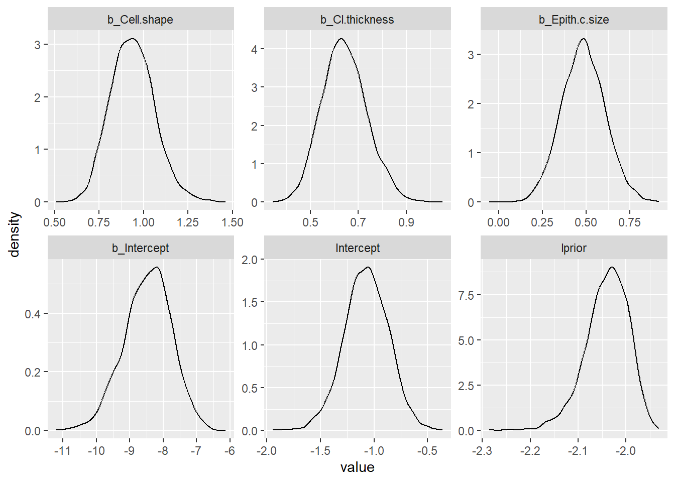
8.3.5 Mixed model with INLA
Plotting world_sfdf to identify characteristics of the data
library(ggplot2)
ggplot(data=world_sfdf, aes(x=LifeExpectancy, y=MeanLifetimeRisk,
              color=Income, shape=Continent))+
  geom_point()+
  geom_jitter()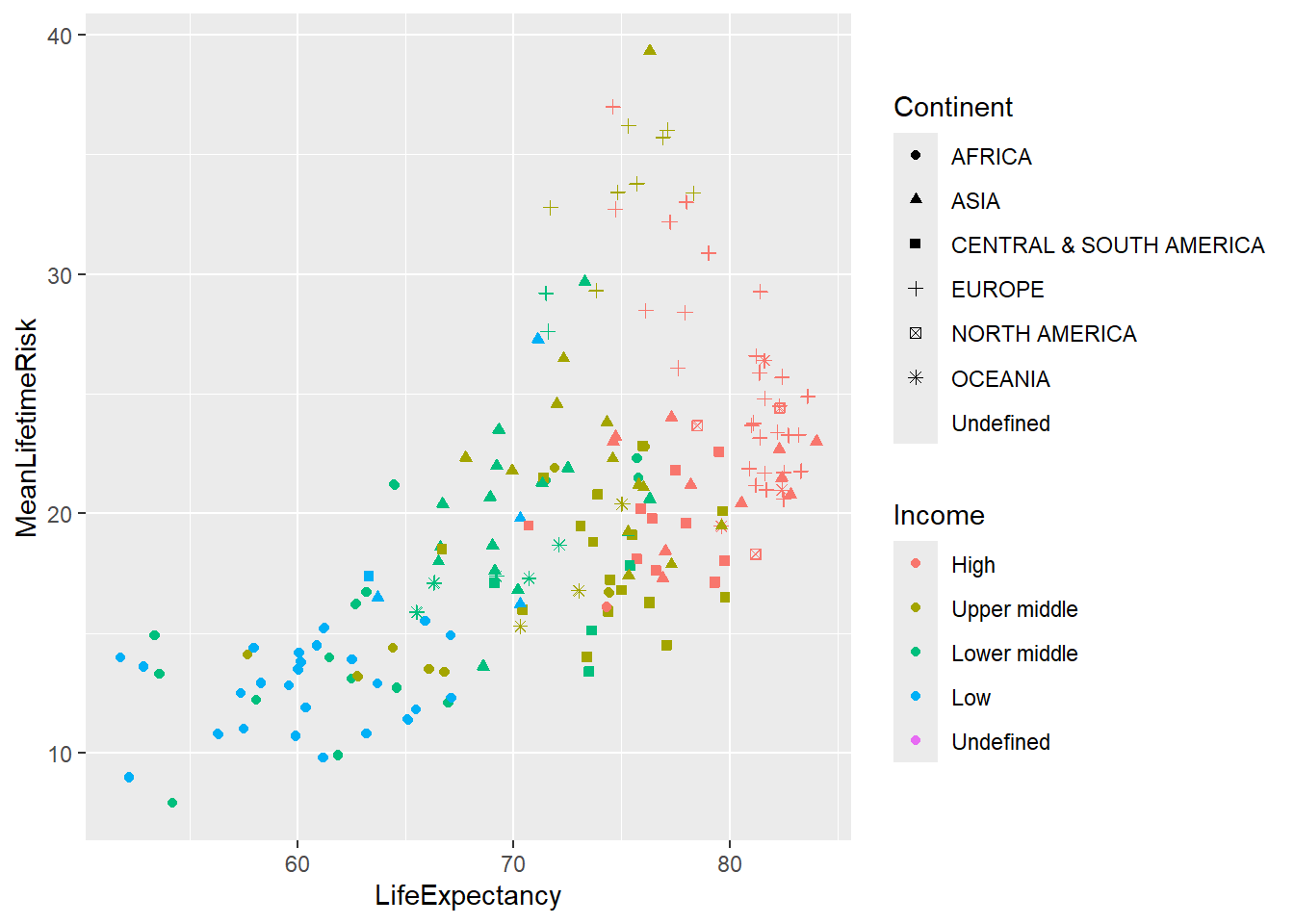
Intercept model with INLA
# Set prior on precision
prec.prior <- list(prec = list(param = c(0.001, 0.001)))

Inla_Income<-inla(MeanLifetimeRisk~1+LifeExpectancy+f(Income,
    model = "iid",
    hyper = prec.prior),
    data =world_sfdf[,c(23,12, 15, 20)],
    control.predictor = list(compute = TRUE))

summary(Inla_Income)
Call:
   c("inla.core(formula = formula, family = family, contrasts = contrasts,
   ", " data = data, quantiles = quantiles, E = E, offset = offset, ", "
   scale = scale, weights = weights, Ntrials = Ntrials, strata = strata,
   ", " lp.scale = lp.scale, link.covariates = link.covariates, verbose =
   verbose, ", " lincomb = lincomb, selection = selection, control.compute
   = control.compute, ", " control.predictor = control.predictor,
   control.family = control.family, ", " control.inla = control.inla,
   control.fixed = control.fixed, ", " control.mode = control.mode,
   control.expert = control.expert, ", " control.hazard = control.hazard,
   control.lincomb = control.lincomb, ", " control.update =
   control.update, control.lp.scale = control.lp.scale, ", "
   control.pardiso = control.pardiso, only.hyperparam = only.hyperparam,
   ", " inla.call = inla.call, inla.arg = inla.arg, num.threads =
   num.threads, ", " keep = keep, working.directory = working.directory,
   silent = silent, ", " inla.mode = inla.mode, safe = FALSE, debug =
   debug, .parent.frame = .parent.frame)" )
Time used:
    Pre = 0.675, Running = 0.469, Post = 0.066, Total = 1.21
Fixed effects:
                 mean    sd 0.025quant 0.5quant 0.975quant   mode   kld
(Intercept)    17.946 2.232      13.42   17.967     22.351 17.965 0.001
LifeExpectancy  0.027 0.019      -0.01    0.027      0.064  0.027 0.000

Random effects:
  Name    Model
    Income IID model

Model hyperparameters:
                                         mean    sd 0.025quant 0.5quant
Precision for the Gaussian observations 0.047 0.004      0.039    0.047
Precision for Income                    0.093 0.069      0.017    0.075
                                        0.975quant  mode
Precision for the Gaussian observations      0.056 0.046
Precision for Income                         0.274 0.046

Marginal log-Likelihood:  -760.87
 is computed
Posterior summaries for the linear predictor and the fitted values are computed
(Posterior marginals needs also 'control.compute=list(return.marginals.predictor=TRUE)')
8.3.6 Mixed model with Stan
Intercept model with BRMS
BRMS_Income <- brm(MeanLifetimeRisk ~ 1 + LifeExpectancy+(1 | Income),
                              data   = world_sfdf,
                              warmup = 100,
                              iter   = 200,
                              chains = 2,
                              inits  = "random",
                              cores  = 2)  #use 2 CPU cores simultaneously instead of just 1.

summary(BRMS_Income)
Plotting of the posterior samples from stan.
post_samples_BRMS_Income <- brms::posterior_samples(BRMS_Income)

post_samples_BRMS_Income %>%
  select(-lp__) %>%
  pivot_longer(cols = everything()) %>%
  ggplot(aes(x = value)) +
  geom_density() +
  facet_wrap(~name, scales = "free")
8.3.7 Metaanalysis with INLA
A Bayesian approach towards metaanalysis is provided below using the package meta4diag (Guo and Riebler 2015). This approach uses the Integrated Nested Laplacian Approximations (INLA). This package has an advantage over the mada package which does not provide a bivariate method for performing summary sensitivity and specificity.
#install.packages("INLA",repos=c(getOption("repos"),INLA="https://inla.r-inla-download.org/R/stable"), dep=TRUE)
library(meta4diag)
Loading required package: gridLoading required package: shinyLoading required package: shinyBSLoading required package: caToolslibrary(INLA)
#data from spot sign metaanalysis
Dat<-read.csv("./Data-Use/ss150718.csv")
#remove duplicates
dat<-subset(Dat, Dat$retain=="yes")
#the data can be viewed under res$data
res <- meta4diag(data = dat)
#perform SROC
SROC(res, crShow = T)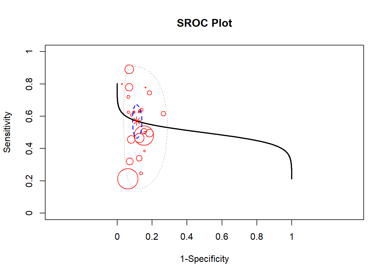
Forest plot of sensitivity using the meta4diag package.
#sensitivity is specified under accuracy.type
#note that there are several different forest plot: mada, metafor, meta4diag
meta4diag::forest(res, accuracy.type="sens", est.type="mean", p.cex="scaled", p.pch=15, p.col="black",
    nameShow="right", dataShow="center", estShow="left", text.cex=1,
    shade.col="gray", arrow.col="black", arrow.lty=1, arrow.lwd=1,
    cut=TRUE, intervals=c(0.025,0.975),
    main="Forest plot of Sensitivity", main.cex=1.5, axis.cex=1)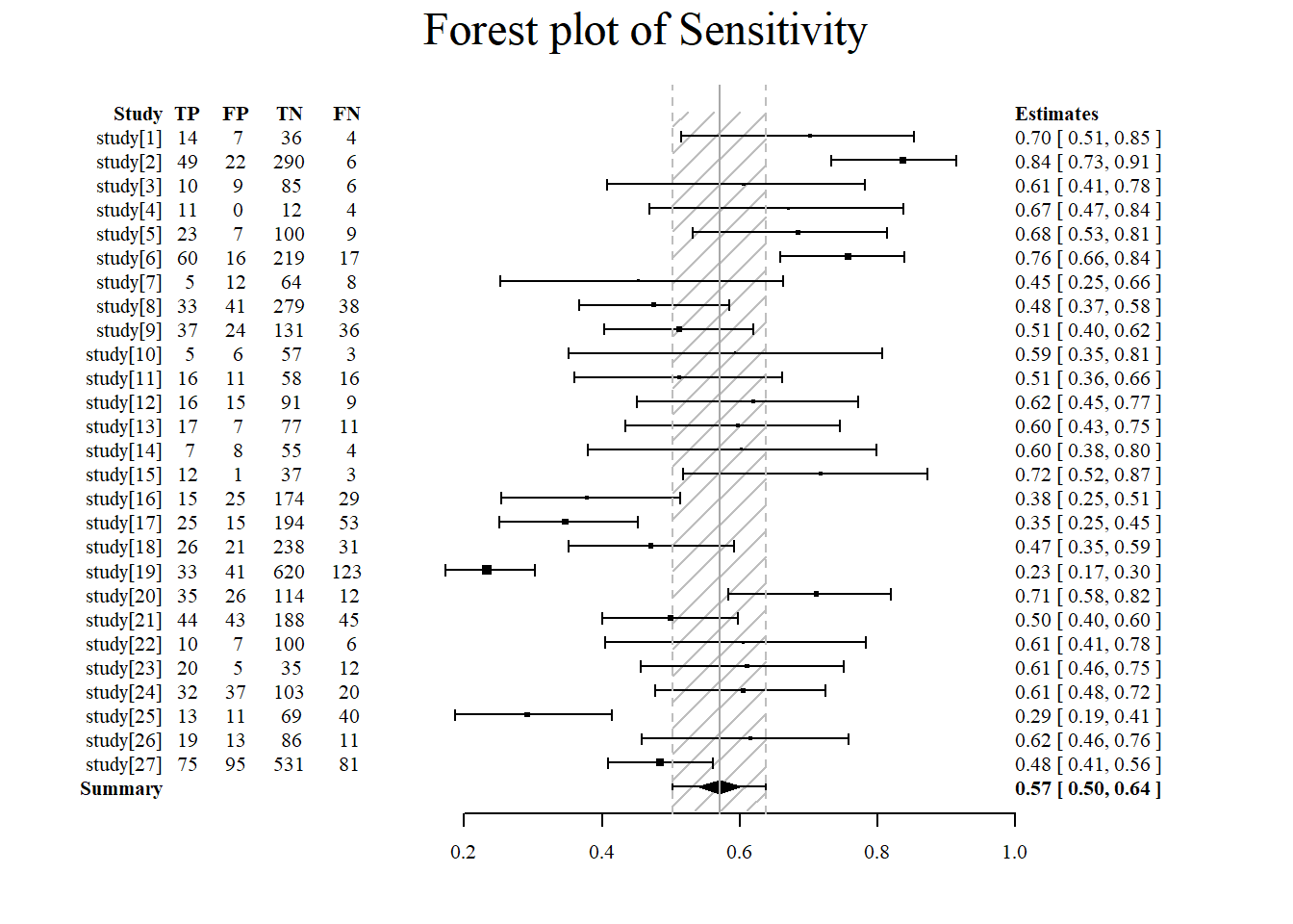
Forest plot of specificity using the meta4diag package.
#specificity is specified under accuracy.type
#note that there are several different forest plot: mada, metafor, meta4diag
meta4diag::forest(res, accuracy.type="spec", est.type="mean", p.cex="scaled", p.pch=15, p.col="black",
    nameShow="right", dataShow="center", estShow="left", text.cex=1,
    shade.col="gray", arrow.col="black", arrow.lty=1, arrow.lwd=1,
    cut=TRUE, intervals=c(0.025,0.975),
    main="Forest plot of Specificity", main.cex=1.5, axis.cex=1)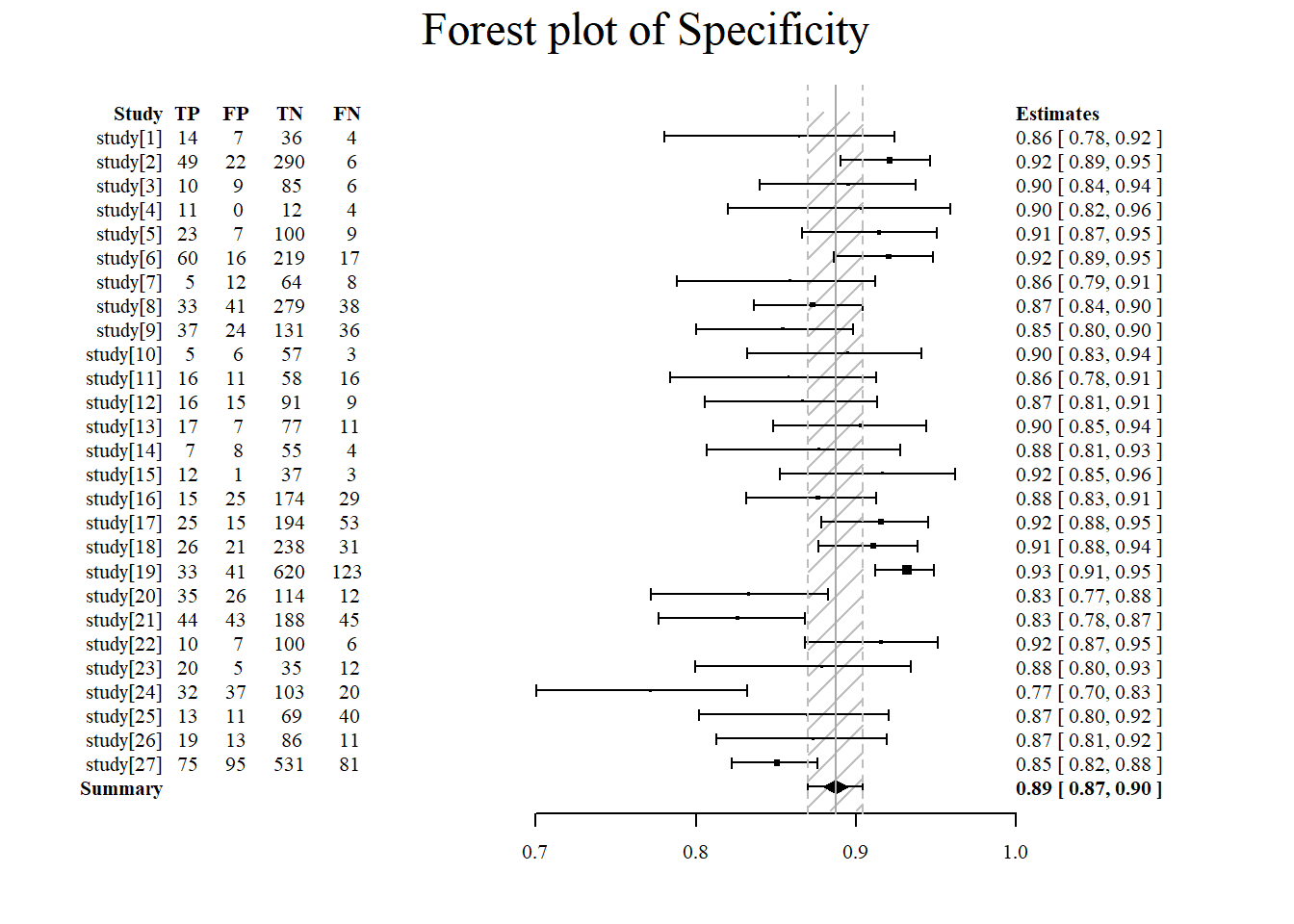
8.3.8 Cost
The example below is provided by hesim.
library("hesim")
Attaching package: 'hesim'The following object is masked from 'package:tidyr':
expandThe following object is masked from 'package:Matrix':
expandlibrary("data.table")
Attaching package: 'data.table'The following objects are masked from 'package:lubridate':
hour, isoweek, mday, minute, month, quarter, second, wday, week,
yday, yearThe following objects are masked from 'package:dplyr':
between, first, lastThe following object is masked from 'package:purrr':
transposestrategies <- data.table(strategy_id = c(1, 2))
n_patients <- 1000
patients <- data.table(patient_id = 1:n_patients,
age = rnorm(n_patients, mean = 70, sd = 10),
female = rbinom(n_patients, size = 1, prob = .4))
states <- data.table(state_id = c(1, 2),
state_name = c("Healthy", "Sick"))
# Non-death health states
tmat <- rbind(c(NA, 1, 2),
c(3, NA, 4),
c(NA, NA, NA))
colnames(tmat) <- rownames(tmat) <- c("Healthy", "Sick", "Dead")
transitions <- create_trans_dt(tmat)
transitions[, trans := factor(transition_id)]
hesim_dat <- hesim_data(strategies = strategies,
patients = patients,
states = states,
transitions = transitions)
print(hesim_dat)$strategies
strategy_id
1: 1
2: 2
$patients
patient_id age female
1: 1 91.34467 0
2: 2 81.69716 0
3: 3 75.29175 1
4: 4 62.43642 1
5: 5 60.60035 0
---
996: 996 78.25143 1
997: 997 67.95121 0
998: 998 88.22978 1
999: 999 76.12606 1
1000: 1000 63.21090 0
$states
state_id state_name
1: 1 Healthy
2: 2 Sick
$transitions
transition_id from to from_name to_name trans
1: 1 1 2 Healthy Sick 1
2: 2 1 3 Healthy Dead 2
3: 3 2 1 Sick Healthy 3
4: 4 2 3 Sick Dead 4
attr(,"class")
[1] "hesim_data"