14  Geospatial analysis

This section deals with the use of geospatial analysis in healthcare. There is a detailed tutorial online available here

14.1 Geocoding

There are several packages avalable for obtaining geocode or longitude and latitude of location. The tmaptools package provide free geocoding using OpenStreetMap or OSM overpass API. Both ggmap and googleway access Google Maps API and will require a key and payment for access.

14.1.1 OpenStreetMap

This is a simple example to obtain the geocode of Monash Medical Centre. However, such a simple example does not always work without the full address. There are other libraries for accessing other data from OSM such as parks, restaurants etc.

library(tmaptools)
mmc<-geocode_OSM ("monash medical centre, clayton")
mmc
$query
[1] "monash medical centre, clayton"

$coords
        x         y 
145.12072 -37.92088 

$bbox
     xmin      ymin      xmax      ymax 
145.12067 -37.92094 145.12077 -37.92083 

The osmdata library includes function opg for extracting data from Overpass query. The list is available at https://wiki.openstreetmap.org/wiki/Map_features#Transportation.

library(tidyverse )
Warning: package 'ggplot2' was built under R version 4.3.3
── Attaching core tidyverse packages ──────────────────────── tidyverse 2.0.0 ──
✔ dplyr     1.1.2     ✔ readr     2.1.4
✔ forcats   1.0.0     ✔ stringr   1.5.0
✔ ggplot2   3.5.1     ✔ tibble    3.2.1
✔ lubridate 1.9.2     ✔ tidyr     1.3.0
✔ purrr     1.0.1     
── Conflicts ────────────────────────────────────────── tidyverse_conflicts() ──
✖ dplyr::filter() masks stats::filter()
✖ dplyr::lag()    masks stats::lag()
ℹ Use the conflicted package (<http://conflicted.r-lib.org/>) to force all conflicts to become errors
library(osmdata)
Data (c) OpenStreetMap contributors, ODbL 1.0. https://www.openstreetmap.org/copyright
library(sf)
Linking to GEOS 3.11.2, GDAL 3.6.2, PROJ 9.2.0; sf_use_s2() is TRUE

Note that getbb now returns an error “HTTP 405 Method Not Allowed”. It seems that there is an error with getbb function.

# build a query
query <- getbb(bbox = "Brisbane, QLD, australia") %>% opq() %>%
  add_osm_feature(key = "amenity", value = "community_centre")

Vector for bbox can be obtained using nominatimlite.

nominatim_polygon <- nominatimlite::geo_lite_sf(address = "Fairfield, NSW, Australia", points_only = FALSE)
bboxsf <- sf::st_bbox(nominatim_polygon)
bboxsf
     xmin      ymin      xmax      ymax 
150.81120 -33.91416 150.99060 -33.82074 

Extracting data on community centre in Brisbane.

query <- bboxsf %>% opq() %>%
  add_osm_feature(key = "amenity", value = "community_centre")
query
$bbox
[1] "-33.9141628,150.8112007,-33.8207365,150.9906033"

$prefix
[1] "[out:xml][timeout:25];\n(\n"

$suffix
[1] ");\n(._;>;);\nout body;"

$features
[1] "[\"amenity\"=\"community_centre\"]"

$osm_types
[1] "node"     "way"      "relation"

attr(,"class")
[1] "list"           "overpass_query"
attr(,"nodes_only")
[1] FALSE

Extracting data on fast food eateries in Brisbane.

query_FF <- bboxsf %>% opq() %>%
  add_osm_feature(key = "amenity", value = "fast_food")
query_FF
$bbox
[1] "-33.9141628,150.8112007,-33.8207365,150.9906033"

$prefix
[1] "[out:xml][timeout:25];\n(\n"

$suffix
[1] ");\n(._;>;);\nout body;"

$features
[1] "[\"amenity\"=\"fast_food\"]"

$osm_types
[1] "node"     "way"      "relation"

attr(,"class")
[1] "list"           "overpass_query"
attr(,"nodes_only")
[1] FALSE

Get information on tags for highway. Wikipedia has a page OpenStreetMap Wiki on highway.

available_tags("highway") %>% head()
# A tibble: 6 × 2
  Key     Value       
  <chr>   <chr>       
1 highway bridleway   
2 highway bus_guideway
3 highway bus_stop    
4 highway busway      
5 highway construction
6 highway corridor    

Use the tags from above to define wide street. Plot the wide street using ggplot2.

wide_streets <- bboxsf%>%
  opq()%>%
  add_osm_feature(key = "highway", 
        value = c("motorway", "primary", "motorway_link", "primary_link", "secondary", "secondary_link")) %>%
  osmdata_sf()

ggplot() +
  geom_sf(data = wide_streets$osm_lines,
          inherit.aes = FALSE,
          color = "black")

Service or lane way can be defined by service.

narrow_streets <- bboxsf%>%
  opq()%>%
  add_osm_feature(key = "highway", 
        value = c("service")) %>%
  osmdata_sf()


ggplot() +
  geom_sf(data = narrow_streets$osm_lines,
          inherit.aes = FALSE,
          color = "blue")

14.1.2 Google Maps API

The equivalent code in ggmap is provided below. Note that a key is required from Google Maps API.

library(ggmap)
register_google(key="Your Key")
#geocode
geocode ("monash medical centre, clayton")

#trip
#mapdist("5 stud rd dandenong","monash medical centre")

The next demonstration is the extraction of geocodes from multiple addresses embedded in a column of data within a data frame. This is more efficient compared to performing geocoding line by line. An example is provided on how to create your own icon on the leaflet document as well as taking a picture for publication.

library(dplyr)
library(tidyr) #unite verb from tidyr
library(readr)
library(tmaptools)
library(leaflet)
library(sf)

clinic<-read_csv("./Data-Use/TIA_clinics.csv")
Rows: 25 Columns: 11
── Column specification ────────────────────────────────────────────────────────
Delimiter: ","
chr (10): City, Country, Setting, Pre-COVID-Assessment, Post-COVID-Assessmen...
dbl  (1): COVID Alert Level

ℹ Use `spec()` to retrieve the full column specification for this data.
ℹ Specify the column types or set `show_col_types = FALSE` to quiet this message.
clinic2<-clinic %>%  
  unite ("address",City:Country,sep = ",")%>%   filter(!is.na(`Clinic-Status`)) 

load("./Data-Use/TIAclinics_geo.Rda")

clinics_geo<-left_join(clinics_geo,clinic2, by=c("query"="address"))
#create icon markers
#icon markers
icons_blue <- awesomeIcons(
  icon= 'medkit',
  iconColor = 'black',
  library = 'ion',
  markerColor = "blue"
)
icons_red <- awesomeIcons(
  icon= 'medkit',
  iconColor = 'black',
  library = 'ion',
  markerColor = "red"
)

#subset 
clinics_geo_active<-clinics_geo %>%filter(`Clinic-Status`=="Active")
clinics_geo_inactive<-clinics_geo %>%filter(`Clinic-Status` !="Active")
m<-leaflet(data=clinics_geo) %>% 
  addTiles() %>% #default is OSM
    addAwesomeMarkers(lat=clinics_geo_active$lat,lng=clinics_geo_active$lon,
          icon=icons_blue,label = ~as.character(clinics_geo_active$query) ) %>%
  addAwesomeMarkers(lat=clinics_geo_inactive$lat,lng=clinics_geo_inactive$lon,
        icon=icons_red,label = ~as.character(clinics_geo_inactive$query)) 

#make pics using mapshot
mapview::mapshot(m, url = paste0(getwd(),
  file="./Data-Use/TIAclinic_world.html"), file = paste0(getwd(), "./Data-Use/TIAclinic_world.png"))
The legacy packages maptools, rgdal, and rgeos, underpinning the sp package,
which was just loaded, will retire in October 2023.
Please refer to R-spatial evolution reports for details, especially
https://r-spatial.org/r/2023/05/15/evolution4.html.
It may be desirable to make the sf package available;
package maintainers should consider adding sf to Suggests:.
The sp package is now running under evolution status 2
     (status 2 uses the sf package in place of rgdal)
m

Googleway has the flexibility of easily interrogating Google Maps API for time of trip and traffic condition.

library(googleway)
key="Your Key"
#trip to MMC
#traffic model can be optimistic, best guess, pessimistic
google_distance("5 stud rd dandenong","monash medical centre", key=key, departure_time=as.POSIXct("2019-12-03 08:15:00 AEST"),traffic_model = "optimistic")

14.2 Sp and sf objects

There are several methods for reading the shapefile data. Previously rgdal library was used. This approach creates files which can be described as S4 object in that there are slots for different data. The spatial feature sf approach is much easier to handle and the data can easily be subset and merged if needed. An example of conversion between sp and sf is provided.

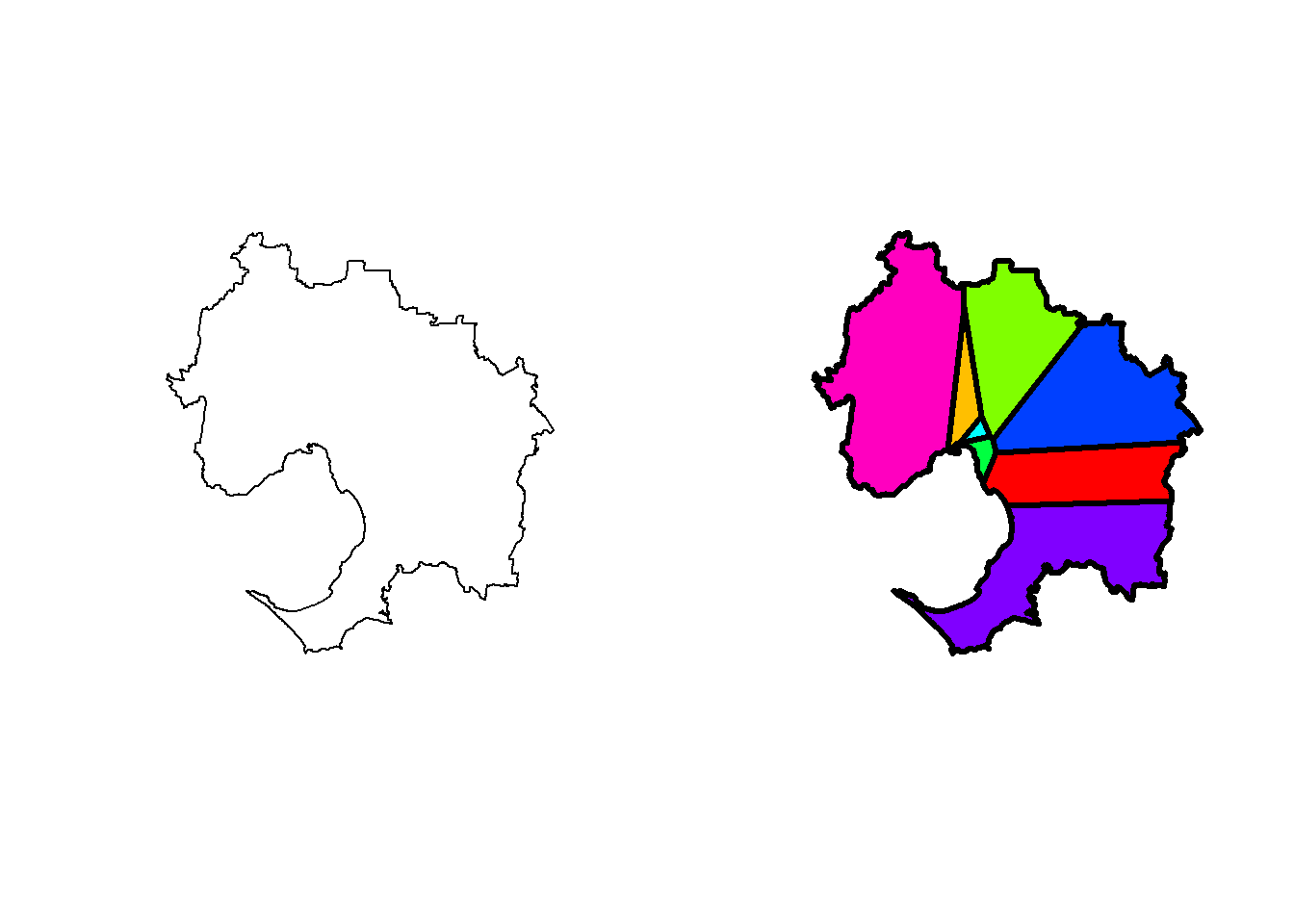
Here, base R plot is used to illustrate the shapefile of Melbourne and after parcellation into Voronois, centred by the hospital location.

library(dismo)
Loading required package: raster
Loading required package: sp

Attaching package: 'raster'
The following object is masked from 'package:dplyr':

    select
library(ggvoronoi)
rgeos version: 0.6-3, (SVN revision 696)
 GEOS runtime version: 3.11.2-CAPI-1.17.2 
 Please note that rgeos will be retired during October 2023,
plan transition to sf or terra functions using GEOS at your earliest convenience.
See https://r-spatial.org/r/2023/05/15/evolution4.html for details.
 GEOS using OverlayNG
 Linking to sp version: 2.0-0 
 Polygon checking: TRUE 
library(tidyverse)
library(sf)

par(mfrow=c(1,2)) #plot 2 objects in 1 row
msclinic<-read.csv("./Data-Use/msclinic.csv") %>% filter(clinic==1, metropolitan==1)

#convert to spatialpointdataframe
coordinates(msclinic) <- c("lon", "lat")
#proj4string(msclinic) <- CRS("+proj=longlat +datum=WGS84")

proj4string(msclinic) <- CRS("+proj=longlat +ellps=GRS80 +towgs84=0,0,0,0,0,0,0 +no_defs")

#create voronoi from msclinic data
#msclinic object is in sp
msv<-voronoi(msclinic)

#create voronoi from msclinic data
#object is in sp
msv<-voronoi(msclinic)

#subset Greater Melbourne
Melb<-st_read("./Data-Use/GCCSA_2016_AUST.shp") %>% filter(STE_NAME16=="Victoria",GCC_NAME16=="Greater Melbourne")
Reading layer `GCCSA_2016_AUST' from data source 
  `C:\Users\phant\Documents\Book\Healthcare-R-Book\Data-Use\GCCSA_2016_AUST.shp' 
  using driver `ESRI Shapefile'
Simple feature collection with 34 features and 5 fields (with 18 geometries empty)
Geometry type: MULTIPOLYGON
Dimension:     XY
Bounding box:  xmin: 96.81694 ymin: -43.74051 xmax: 167.998 ymax: -9.142176
Geodetic CRS:  GDA94
#transform sf to sp object
Melb<-as(Melb,Class="Spatial")
plot(Melb)

#voronoi bound by greater melbourne
vor <- dismo::voronoi(msclinic, ext=extent(Melb))

#intersect is present in base R, dplyr, raster, lubridate etc
r <- raster::intersect(vor, Melb)

#r<-intersect(msv,gccsa_fsp)

#
msclinic$hospital<-as.character(msclinic$hospital)
plot(r, col=rainbow(length(r)), lwd=3)

#sp back to sf
#error with epsg conversion back
msclinic_sf<-st_as_sf(msclinic,crs=4283)

14.2.0.1 Brisbane

Obtain the Brisbane data as sf object.

ComCentre <- osmdata::osmdata_sf(query)
names(ComCentre$osm_points)
 [1] "osm_id"           "name"             "addr:city"        "addr:housenumber"
 [5] "addr:postcode"    "addr:state"       "addr:street"      "amenity"         
 [9] "community_centre" "level"            "opening_hours"    "operator"        
[13] "phone"            "website"          "geometry"        

Extract the centroid and polygons. Check that the coordinate reference system is EPSG 4326 or World Geodetic System (WGS) 84.

ComPoint<-ComCentre$osm_points %>% filter(amenity=="community_centre")

ComPoly <- ComCentre$osm_polygons %>%
  st_centroid()
Warning: st_centroid assumes attributes are constant over geometries
Com <- bind_rows(ComPoly, ComPoint)
st_crs(Com)
Coordinate Reference System:
  User input: EPSG:4326 
  wkt:
GEOGCRS["WGS 84",
    ENSEMBLE["World Geodetic System 1984 ensemble",
        MEMBER["World Geodetic System 1984 (Transit)"],
        MEMBER["World Geodetic System 1984 (G730)"],
        MEMBER["World Geodetic System 1984 (G873)"],
        MEMBER["World Geodetic System 1984 (G1150)"],
        MEMBER["World Geodetic System 1984 (G1674)"],
        MEMBER["World Geodetic System 1984 (G1762)"],
        ELLIPSOID["WGS 84",6378137,298.257223563,
            LENGTHUNIT["metre",1]],
        ENSEMBLEACCURACY[2.0]],
    PRIMEM["Greenwich",0,
        ANGLEUNIT["degree",0.0174532925199433]],
    CS[ellipsoidal,2],
        AXIS["geodetic latitude (Lat)",north,
            ORDER[1],
            ANGLEUNIT["degree",0.0174532925199433]],
        AXIS["geodetic longitude (Lon)",east,
            ORDER[2],
            ANGLEUNIT["degree",0.0174532925199433]],
    USAGE[
        SCOPE["Horizontal component of 3D system."],
        AREA["World."],
        BBOX[-90,-180,90,180]],
    ID["EPSG",4326]]

Plot the map of community centres in Ballarat with tmap. The view argument in tmap_mode set this plotting to interactive viewing with tmap with leaflet. The leaflet library can be called directly using tmap_leaflet

#extract bounding box for Brisbane

#Brisbane <- osmdata::getbb("Brisbane, australia", format_out = "sf_polygon")$multipolygon 

Brisbane<-nominatim_polygon$geometry

library(tmap)

#set interactive view
tmap_mode("view")
tmap mode set to interactive viewing
#plot outline of Ballarat
  tm_shape(Brisbane)+
 tm_borders()+

  #plot community centres
tm_shape(Com) +
  tm_dots()

14.3 Thematic map

In the first chapter we provided thematic map examples with ggplot2, tmap and plotly.

14.3.0.1 Finland

Here we will illustrate with mapview library using open data on Finland. Mapbox is another library that can be used but that library requires registration.

library(geofi)
library(ggplot2)
library(tmap)
library(tidyverse)

library(tidyr)
library(pxweb)
pxweb 0.16.2: R tools for the PX-WEB API.
https://github.com/ropengov/pxweb
library(janitor)

Attaching package: 'janitor'
The following object is masked from 'package:raster':

    crosstab
The following objects are masked from 'package:stats':

    chisq.test, fisher.test
#data  on Finland
#https://pxnet2.stat.fi/PXWeb/pxweb/en/Kuntien_avainluvut/
#Kuntien_avainluvut__2021/kuntien_avainluvut_2021_viimeisin.px/table/
#tableViewLayout1/
FinPop<-readxl::read_xlsx("./Data-Use/Kuntien avainluvut_20210704-153529.xlsx", skip = 2)
New names:
• `` -> `...1`
FinPop2<-FinPop[-c(1),] #remove data for entire Finland

#get shapefile for municipality
municipalities <- get_municipalities(year = 2020, scale = 4500) #sf object)
Requesting response from: http://geo.stat.fi/geoserver/wfs?service=WFS&version=1.0.0&request=getFeature&typename=tilastointialueet%3Akunta4500k_2020
Warning: Coercing CRS to epsg:3067 (ETRS89 / TM35FIN)
Data is licensed under: Attribution 4.0 International (CC BY 4.0)
#join shapefile and population data
municipalities2<-right_join(municipalities, FinPop2, by=c("name"="...1")) %>%
  rename(Pensioner=`Proportion of pensioners of the population, %, 2019`,Age65=`Share of persons aged over 64 of the population, %, 2020`) %>% na.omit()

#plot map using mapview
mapview::mapview(municipalities2["Age65"],layer.name="Age65")

This example illustrates how to add arguments in mapview

library(mapview)
library(sf)
library(tmaptools)

#NY Shape file
NYsf<-st_read("./Data-Use/Borough_Boundaries/geo_export_7d3b2726-20d8-4aa4-a41f-24ba74eb6bc0.shp")
Reading layer `geo_export_7d3b2726-20d8-4aa4-a41f-24ba74eb6bc0' from data source `C:\Users\phant\Documents\Book\Healthcare-R-Book\Data-Use\Borough_Boundaries\geo_export_7d3b2726-20d8-4aa4-a41f-24ba74eb6bc0.shp' 
  using driver `ESRI Shapefile'
Simple feature collection with 5 features and 4 fields
Geometry type: MULTIPOLYGON
Dimension:     XY
Bounding box:  xmin: -74.25559 ymin: 40.49612 xmax: -73.70001 ymax: 40.91553
Geodetic CRS:  WGS84(DD)
#NY subway -does not go to Staten Island
NYsubline<-st_read("./Data-Use/NYsubways/geo_export_147781bc-e472-4c12-8cd2-5f9859f90706.shp")
Reading layer `geo_export_147781bc-e472-4c12-8cd2-5f9859f90706' from data source `C:\Users\phant\Documents\Book\Healthcare-R-Book\Data-Use\NYsubways\geo_export_147781bc-e472-4c12-8cd2-5f9859f90706.shp' 
  using driver `ESRI Shapefile'
Simple feature collection with 742 features and 6 fields
Geometry type: LINESTRING
Dimension:     XY
Bounding box:  xmin: -74.03088 ymin: 40.57559 xmax: -73.75541 ymax: 40.90312
Geodetic CRS:  WGS84(DD)
#NY subway stations
NYsubstation<-st_read("./Data-Use/NYsubways/geo_export_0dab2fcf-79b8-409a-b940-7c98778a4418.shp")
Reading layer `geo_export_0dab2fcf-79b8-409a-b940-7c98778a4418' from data source `C:\Users\phant\Documents\Book\Healthcare-R-Book\Data-Use\NYsubways\geo_export_0dab2fcf-79b8-409a-b940-7c98778a4418.shp' 
  using driver `ESRI Shapefile'
Simple feature collection with 473 features and 5 fields
Geometry type: POINT
Dimension:     XY
Bounding box:  xmin: -74.03088 ymin: 40.57603 xmax: -73.7554 ymax: 40.90313
Geodetic CRS:  WGS84(DD)
#list of NY hospitals
Hosp<-c("North Shore University Hospital","Long Island Jewish Medical Centre","Staten Island University Hospital","Lennox Hill Hospital","Long Island Jewish Forest Hills","Long Island Jewish Valley Stream","Plainview Hospital","Cohen Children's Medical Center","Glen Cove Hospital","Syosset Hospital")

#geocode NY hospitals and return sf object
Hosp_geo<-geocode_OSM(paste0(Hosp,",","New York",",","USA"),as.sf = TRUE)
No results found for "Long Island Jewish Medical Centre,New York,USA".
No results found for "Lennox Hill Hospital,New York,USA".
#data from jama paper on variation in mortality from covid
mapview(NYsf, zcol="boro_name")+
  mapview(NYsubline, zol="name")+
    #cex is the circle size default=6
    mapview(NYsubstation, zol="line",cex=1)+
      mapview(Hosp_geo, zcol="query", cex=3)

14.3.0.2 Denmark

The example shown under Data wrangling on how to extract data from pdf is now put to use to create thematic map of stroke number per region in Denmark.

library(dplyr)
library(tidyverse)
library(sf)
library(eurostat)
library(leaflet)
library(mapview)
library(tmaptools)

#####################code to generate HospLocations.Rda
load ("./Data-Use/europeRGDK.Rda")

#create data on hospitals
#hosp_addresses <- c(
#  AarhusHospital = "aarhus university hospital, aarhus, Denmark",
#  AalborgHospital = "Hobrovej 18-22 9100 aalborg, Denmark",
#  HolstebroHospital = "Lægårdvej 12 7500 Holstebro, Holstebro, Denmark",   VejleHospital="Vejle Sygehus,Beriderbakken 4, Vejle, Denmark",
#  EsbjergHospital="Esbjerg Sygehus, Esbjerg, Denmark",
#SoenderborgHospital="Sydvang 1C 6400 Sønderborg, Denmark",
#OdenseHospital="Odense Sygehus, Odense, Denmark",   
#RoskildeHospital="Roskilde Sygehus,  Roskilde, Denmark",  
#BlegdamsvejHospital="Rigshospitalet blegdamsvej, 9 Blegdamsvej, København, Denmark",  
#GlostrupHospital="Rigshospitalet Glostrup, Glostrup, Denmark")

#geocode hospitals using OpenStreetMap. This function works better with street addresses
#HospLocations <- tmaptools::geocode_OSM(hosp_addresses, as.sf=TRUE)

#convert data into sf object
#HospLocations <- sf::st_transform(HospLocations,           sf::st_crs(europeRGDK)) 

#CSC comprehensive stroke centre
#PSC primary stroke centre
#HospLocations$Center<-c("CSC", "PSC", "PSC", "PSC", "PSC", "PSC", "CSC", "PSC", "CSC", "PSC")

#save HospLocations
#save(HospLocations, "HospLocations.Rda")

load("./Data-Use/HospLocations.Rda")

##https://ec.europa.eu/eurostat/web/nuts/background
load("./Data-Use/euro_nuts2_sf.Rda")
DKnuts2_sf<- euro_nuts2_sf%>% filter(str_detect(NUTS_ID,"^DK"))
old-style crs object detected; please recreate object with a recent sf::st_crs()
#convert pdf to csv file
dk<-read.csv("./Data-Use/denmarkstrokepdf.csv")

#extract only data on large regions=NUTS2
dk2<-dk[c(4:8),]

#clean up column X.1 containing stroke data
#remove numerator before back slash then remove number before slash sign
dk2$strokenum<-str_replace(dk2$X.1,"[0-9]*","") %>%
  str_replace("/","\\") %>% as.numeric()
dk2$Uoplyst<-str_replace(dk2$Uoplyst,"Sjælland","Sjælland")

#merge sf file for DK nuts2 with stroke number
DKnuts2_sf2<-right_join(DKnuts2_sf,dk2,by=c("NUTS_NAME"="Uoplyst"))

#add population from Statistics Denmark 2018 
DKnuts2_sf2$pop<-c(589148,1822659,835024, 1313596,1220763)
DKnuts2_sf2$male<-c(297679,894553,416092,657817,610358)
DKnuts2_sf2$maleper<-round(with(DKnuts2_sf2,pop/male),2)

#plot map
mapview(DKnuts2_sf2["strokenum"], layer.name="Stroke Number") +mapview(HospLocations, zcol="Center", layer.name="Hospital Designation")
old-style crs object detected; please recreate object with a recent sf::st_crs()

14.3.1 Calculate distance to Hospital-OpenStreetMap

Determine distance from hospital to centroid of kommunes rather than the larger regions of Denmark. This can be performed with OpenStreetMap or Google Maps API.

dist_to_loc <- function (geometry, location){
    units::set_units(st_distance(st_centroid (geometry), location)[,1], km)
}

Perform the analysis.

load ("./Data-Use/europeRGDK.Rda")

#set distance 10 km
#change to 100 km
dist_range <- units::set_units(100, km)

##
europeRGDK <- mutate(europeRGDK,
       DirectDistanceToAarhus = dist_to_loc(geometry,HospLocations["AarhusHospital", ]),
       DirectDistanceToAalborg     = dist_to_loc(geometry,HospLocations["AalborgHospital", ]),
       DirectDistanceToHolstebro     = dist_to_loc(geometry,HospLocations["HolstebroHospital", ]),
       DirectDistanceToVejle     = dist_to_loc(geometry,HospLocations["VejleHospital", ]),
       DirectDistanceToEsbjerg     = dist_to_loc(geometry,HospLocations["EsbjergHospital", ]),
       DirectDistanceToSoenderborg = dist_to_loc(geometry,HospLocations["SoenderborgHospital", ]),
       DirectDistanceToOdense     = dist_to_loc(geometry,HospLocations["OdenseHospital", ]),
       DirectDistanceToRoskilde     = dist_to_loc(geometry,HospLocations["RoskildeHospital", ]),
       DirectDistanceToBlegdamsvej     = dist_to_loc(geometry,HospLocations["BlegdamsvejHospital", ]),
       DirectDistanceToGlostrup     = dist_to_loc(geometry,HospLocations["GlostrupHospital", ]),
       #
       DirectDistanceToNearest   = pmin(DirectDistanceToAarhus,
      DirectDistanceToAalborg,DirectDistanceToHolstebro,
      DirectDistanceToVejle,DirectDistanceToEsbjerg, DirectDistanceToSoenderborg,DirectDistanceToOdense,
      DirectDistanceToRoskilde,DirectDistanceToBlegdamsvej,
      DirectDistanceToGlostrup))
old-style crs object detected; please recreate object with a recent sf::st_crs()
StrokeHosp <- filter(europeRGDK,                                               DirectDistanceToNearest < dist_range) %>%
        mutate(Postcode = as.numeric(COMM_ID)) 
old-style crs object detected; please recreate object with a recent sf::st_crs()
head(StrokeHosp)
Simple feature collection with 6 features and 15 fields
Geometry type: MULTIPOLYGON
Dimension:     XY
Bounding box:  xmin: 8.709358 ymin: 56.83344 xmax: 8.940572 ymax: 56.98483
Geodetic CRS:  +proj=longlat +ellps=GRS80 +no_defs
        COMM_ID Shape_Leng   Shape_Area                       geometry
1 DK10817738668  0.3605216 0.0030530589 MULTIPOLYGON (((8.940572 56...
2 DK10817738669  0.1539856 0.0012336619 MULTIPOLYGON (((8.908073 56...
3 DK10817738670  0.1630955 0.0009363543 MULTIPOLYGON (((8.886687 56...
4 DK10817738671  0.2010890 0.0019239206 MULTIPOLYGON (((8.822215 56...
5 DK10817738672  0.1926252 0.0011456026 MULTIPOLYGON (((8.750229 56...
6 DK10817738673  0.1793186 0.0011254477 MULTIPOLYGON (((8.83318 56....
  DirectDistanceToAarhus DirectDistanceToAalborg DirectDistanceToHolstebro
1          117.7155 [km]           68.11356 [km]             64.41291 [km]
2          115.7763 [km]           65.96041 [km]             64.48420 [km]
3          114.0335 [km]           67.75456 [km]             60.72506 [km]
4          118.1121 [km]           73.63410 [km]             59.09770 [km]
5          119.4927 [km]           76.87186 [km]             57.33305 [km]
6          114.0855 [km]           72.38971 [km]             55.92370 [km]
  DirectDistanceToVejle DirectDistanceToEsbjerg DirectDistanceToSoenderborg
1         140.9514 [km]           163.4109 [km]               230.7453 [km]
2         139.8147 [km]           163.2912 [km]               229.6966 [km]
3         136.7127 [km]           159.5629 [km]               226.5046 [km]
4         138.2621 [km]           158.3096 [km]               227.7350 [km]
5         138.0619 [km]           156.6019 [km]               227.3109 [km]
6         134.1065 [km]           154.9979 [km]               223.6369 [km]
  DirectDistanceToOdense DirectDistanceToRoskilde DirectDistanceToBlegdamsvej
1          195.3515 [km]            245.3869 [km]               266.3579 [km]
2          193.8254 [km]            243.2411 [km]               264.1433 [km]
3          191.2311 [km]            242.1564 [km]               263.3819 [km]
4          193.8937 [km]            246.9101 [km]               268.4274 [km]
5          194.3217 [km]            248.7312 [km]               270.4758 [km]
6          189.6643 [km]            243.1370 [km]               264.8318 [km]
  DirectDistanceToGlostrup DirectDistanceToNearest Postcode
1            258.4642 [km]           64.41291 [km]    28310
2            256.2729 [km]           64.48420 [km]    28311
3            255.3919 [km]           60.72506 [km]    28312
4            260.3345 [km]           59.09770 [km]    28313
5            262.3009 [km]           57.33305 [km]    28314
6            256.6704 [km]           55.92370 [km]    28315

14.4 Spatial regression

This is data published in Jama 29/4/2020 on COVD-19 in New York. The New York borough shapefiles were obtained from New York Open Data at https://data.cityofnewyork.us/City-Government/Borough-Boundaries/tqmj-j8zm. For those wishing to evaluate other datasets, there’s lung and lip cancer data in SpatialEpi library, leukemia in DClusterm library. Key aspect of spatial regression is that neighbouring regions are similar and distant regions are less so. It uses the polyn2nb in spdep library to create the neighbourhood weight. The map of residual for the New York data does not suggest spatial association of residuals.

The Moran’s I is used to test for global spatial autocorrelation among adjacent regions in multidimensional space. Moran’s I requires calculation of neighbourhood. It is related to the number of regions and sum of all spatial weights.

14.4.1 New York COVID-19 mortality

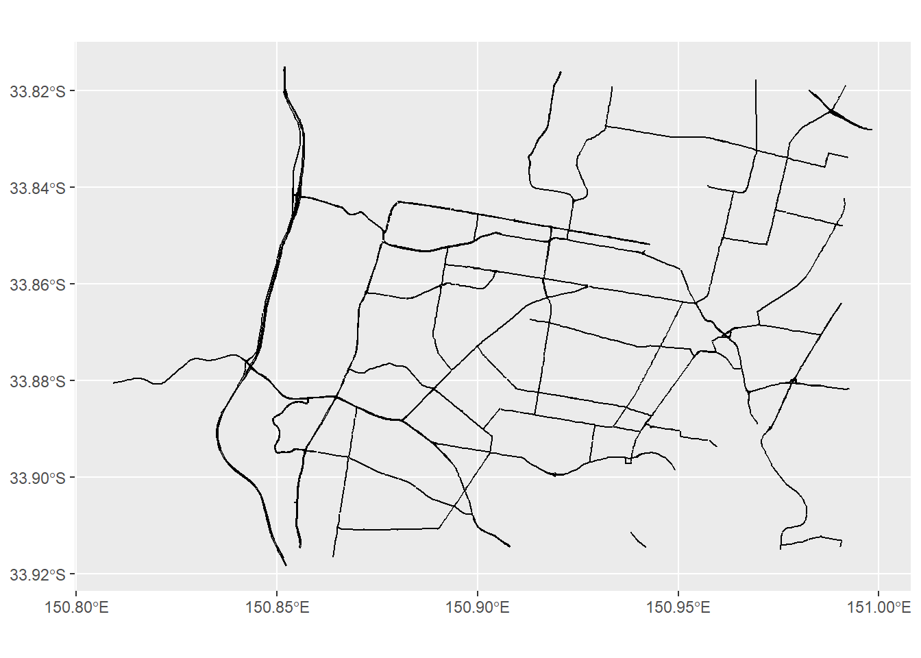
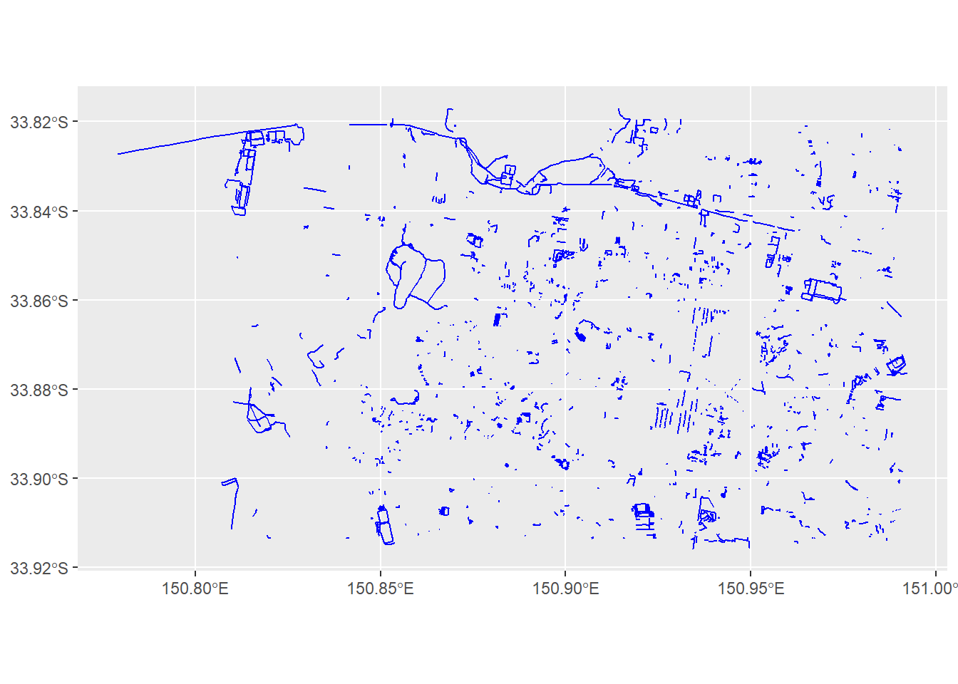
The example below illustrate the need to look at the data. It is not possible to perform spatial regression given the small size of the areal data (4 connected boroughs); Staten Island does not have adjoining border with the others nor share subway system. An intriguing possibility is that areal data analysis at the neighbourhood level would allow a granular examination of socioeconomic effect of COVID-19 on mortality data. To plot the railway lines with tmap the argument tm_lines is required whereas the argument tm_polygons is better suited for plotting the shape file. It

library(leaflet)
library(SpatialEpi)
library(spdep)
Loading required package: spData
To access larger datasets in this package, install the spDataLarge
package with: `install.packages('spDataLarge',
repos='https://nowosad.github.io/drat/', type='source')`
library(spatialreg) #some of spdep moved to spatialreg
Loading required package: Matrix

Attaching package: 'Matrix'
The following objects are masked from 'package:tidyr':

    expand, pack, unpack

Attaching package: 'spatialreg'
The following objects are masked from 'package:spdep':

    get.ClusterOption, get.coresOption, get.mcOption,
    get.VerboseOption, get.ZeroPolicyOption, set.ClusterOption,
    set.coresOption, set.mcOption, set.VerboseOption,
    set.ZeroPolicyOption
library(tidyverse)
library(tmap)
library(sf)
library(dplyr)
library(MASS)

Attaching package: 'MASS'
The following objects are masked from 'package:raster':

    area, select
The following object is masked from 'package:dplyr':

    select
dfj<-data.frame(
Borough=c("Bronx","Brooklyn","Manhattan","Queens","Staten Island"),
Pop=c(1432132,2582830,1628701,2278906,476179),
Age65=c(12.8,13.9,16.5,15.7,16.2),
White=c(25.1,46.6,59.2,39.6,75.1),
Hispanic=c(56.4,19.1,25.9,28.1,18.7),
Afro.American=c(38.3,33.5,16.9,19.9,11.5),
Asian=c(4.6,13.4,14,27.5,11),
Others=c(36.8,10.4,15.4,17,5.2),
Income=c(38467,61220,85066,69320,82166),
Beds=c(336,214,534,144,234),
COVIDtest=c(4599,2970,2844,3800,5603),
COVIDhosp=c(634,400,331,560,370),
COVIDdeath=c(224,181,122,200,143),
COVIDdeathlab=c(173,132,91,154,117),
Diabetes=c(16,27,15,22,25),
Obesity=c(32,12,8,11,8),
Hypertension=c(36,29,23,28,25)) %>% 
  #reverse prevalence per 100000 to raw
  mutate(Age65raw=round(Age65/100*Pop,0),
               Bedsraw=round(Beds/100000*Pop,0),
               COVIDtestraw=round(COVIDtest/100000*Pop,0),
               COVIDhospraw=round(COVIDhosp/100000*Pop,0),
               COVIDdeathraw=round(COVIDdeath/100000*Pop),0)
#Expected
rate<-sum(dfj$COVIDdeathraw)/sum(dfj$Pop)
dfj$Expected<-with(dfj, Pop*rate )

#SMR standardised mortality ratio
dfj$SMR<-with(dfj, COVIDdeathraw/Expected)

#NY Shape file - see this file open from above chunk
NYsf<-st_read("./Data-Use/Borough_Boundaries/geo_export_7d3b2726-20d8-4aa4-a41f-24ba74eb6bc0.shp")
Reading layer `geo_export_7d3b2726-20d8-4aa4-a41f-24ba74eb6bc0' from data source `C:\Users\phant\Documents\Book\Healthcare-R-Book\Data-Use\Borough_Boundaries\geo_export_7d3b2726-20d8-4aa4-a41f-24ba74eb6bc0.shp' 
  using driver `ESRI Shapefile'
Simple feature collection with 5 features and 4 fields
Geometry type: MULTIPOLYGON
Dimension:     XY
Bounding box:  xmin: -74.25559 ymin: 40.49612 xmax: -73.70001 ymax: 40.91553
Geodetic CRS:  WGS84(DD)
#join dataset
NYsf<-left_join(NYsf, dfj,by=c("boro_name"="Borough"))

#contiguity based neighbourhood
NY.nb<-poly2nb(NYsf) 
is.symmetric.nb(NY.nb) # TRUE
[1] TRUE
#NY subway 
NYsubline<-st_read("./Data-Use/NYsubways/geo_export_147781bc-e472-4c12-8cd2-5f9859f90706.shp")
Reading layer `geo_export_147781bc-e472-4c12-8cd2-5f9859f90706' from data source `C:\Users\phant\Documents\Book\Healthcare-R-Book\Data-Use\NYsubways\geo_export_147781bc-e472-4c12-8cd2-5f9859f90706.shp' 
  using driver `ESRI Shapefile'
Simple feature collection with 742 features and 6 fields
Geometry type: LINESTRING
Dimension:     XY
Bounding box:  xmin: -74.03088 ymin: 40.57559 xmax: -73.75541 ymax: 40.90312
Geodetic CRS:  WGS84(DD)
#raw data
tm_shape(NYsf) + 
  tm_polygons(col='SMR',title='COVID raw') +
  tm_shape(NYsubline)+tm_lines(col='name')

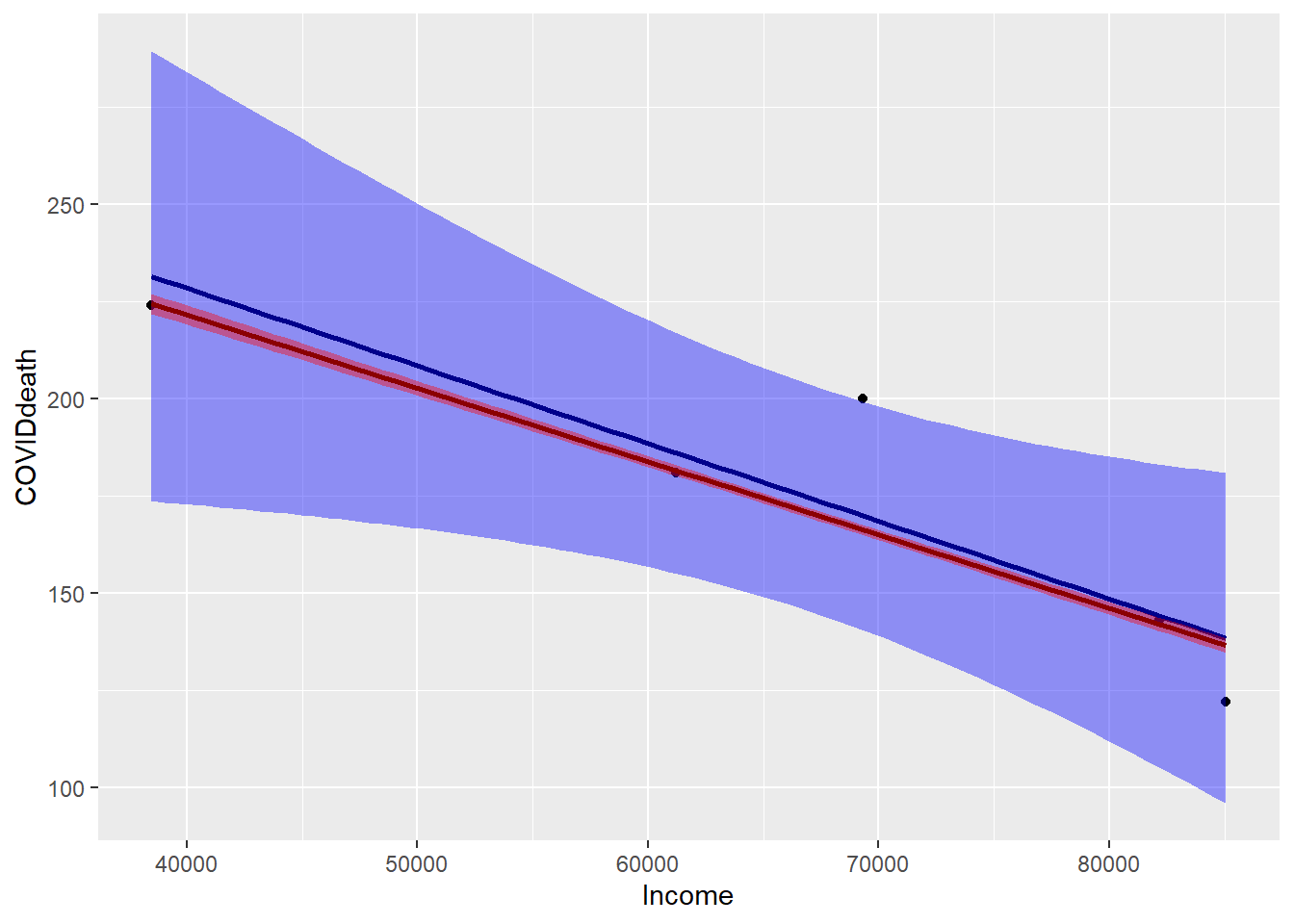
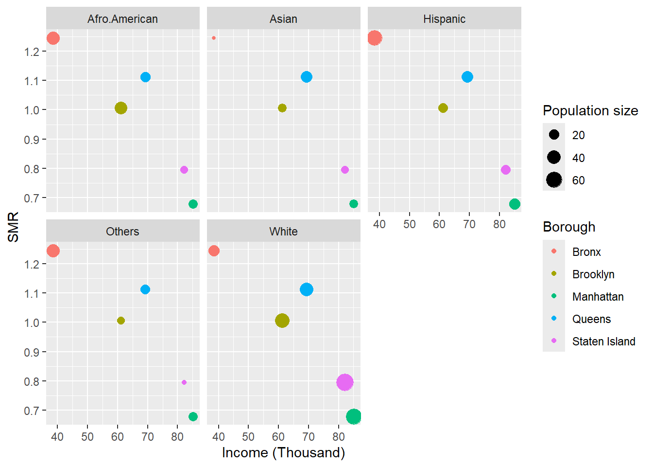
The standardized mortality ratio (ratio of mortality divided by expected value for each borough) for the boroughs were: Bronx (1.245), Brooklyn (1.006), Manhattan (0.678) Queens (1.111) and Staten Island (0.794). The Figure shows a strong relationship between standardized mortality ratio and Income (R2=0.816).

#plot regression lines linear vs robust linear
ggplot(data=NYsf,aes(x=Income,y=COVIDdeath)) + geom_point() + geom_smooth(method='lm',col='darkblue',fill='blue') + geom_smooth(method='rlm',col='darkred',fill='red')
`geom_smooth()` using formula = 'y ~ x'

Standardized mortality ratio and Income among different ethnic groups in Boroughs of New York.

#varies by ethinicty
dfj_long<-pivot_longer(data=dfj, names_to = "Ethnicity", values_to = "Popsize",cols=c(White,Afro.American,Asian,Hispanic,Others))

commonplot<-list(
  scale_size_continuous(name = "Population size"),xlab("Income (Thousand)"),facet_wrap(~Ethnicity,nrow=2)
)
ggplot(data=dfj_long, mapping=aes(x=Income/1000, y=SMR, size=Popsize,colour=Borough))+geom_point()+commonplot

Robust regression to obtain residual for plotting with thematic maps.

#robust linear models
NYsf$resids <- rlm(COVIDdeathraw~Pop+Age65raw,data=NYsf)$res

#tmap robust linear model-residual
#plot using color blind argument
par(mfrow=c(2,1))
tm_shape(NYsf) + tm_polygons(col='resids',title='Residuals')
Variable(s) "resids" contains positive and negative values, so midpoint is set to 0. Set midpoint = NA to show the full spectrum of the color palette.
tm_shape(NYsf) + tm_polygons(col='resids',title='Residuals')+
  tm_style("col_blind")
Variable(s) "resids" contains positive and negative values, so midpoint is set to 0. Set midpoint = NA to show the full spectrum of the color palette.
#create spatial weights for neighbour lists
r.id<-attr(NYsf,"region.id")
lw <- nb2listw(NY.nb,zero.policy = TRUE) #W=row standardised

In this example, the Moran’s I test suggest that the null test can be rejected. This implies random distribution of stroke across the regions of Denmark.

#globaltest spatial autocorrelation using Moran I test from spdep
gm<-moran.test(NYsf$SMR,listw = lw , na.action = na.omit, zero.policy = T)
gm

    Moran I test under randomisation

data:  NYsf$SMR  
weights: lw  n reduced by no-neighbour observations
  

Moran I statistic standard deviate = 0.12086, p-value = 0.4519
alternative hypothesis: greater
sample estimates:
Moran I statistic       Expectation          Variance 
      -0.31010080       -0.33333333        0.03694814 

There’s no evidence of spatial autocorrelation at local level. Note that this data is too small and may not be the ideal to evaluate local Moran’s.

#local test of autocorrelation
lm<-localmoran(NYsf$SMR,listw = nb2listw(NY.nb, 
          zero.policy = TRUE, 
          style = "C") , 
          na.action = na.omit, zero.policy = T)

lm
           Ii         E.Ii      Var.Ii        Z.Ii Pr(z != E(Ii))
1 -0.37737978 -0.362800450 0.264360322 -0.02835563      0.9773785
2  0.00000000  0.000000000 0.000000000         NaN            NaN
3 -0.05282102 -0.007107618 0.009392627 -0.47168273      0.6371533
4  0.03765408 -0.147207581 0.086099458  0.63000884      0.5286888
5 -1.25295769 -0.588823897 0.199930608 -1.48530599      0.1374628
attr(,"call")
localmoran(x = NYsf$SMR, listw = nb2listw(NY.nb, zero.policy = TRUE, 
    style = "C"), zero.policy = T, na.action = na.omit)
attr(,"class")
[1] "localmoran" "matrix"     "array"     
attr(,"quadr")
       mean    median     pysal
1  High-Low  High-Low  High-Low
2   Low-Low   Low-Low   Low-Low
3  High-Low   Low-Low  High-Low
4 High-High High-High High-High
5  Low-High  Low-High  Low-High

14.4.2 Danish Stroke Registry

We now return to spatial regression with the data from Danish stroke registry described above. First we will calculate the SMR

library(tmap)
#Expected
rate<-sum(DKnuts2_sf2$strokenum)/sum(DKnuts2_sf2$pop)
DKnuts2_sf2$Expected<-with(DKnuts2_sf2, pop*rate )

#SMR standardised mortality ratio
DKnuts2_sf2$SMR<-with(DKnuts2_sf2, strokenum/Expected)

tm_shape(DKnuts2_sf2) + 
  tm_polygons(col='SMR',title='Stroke') 

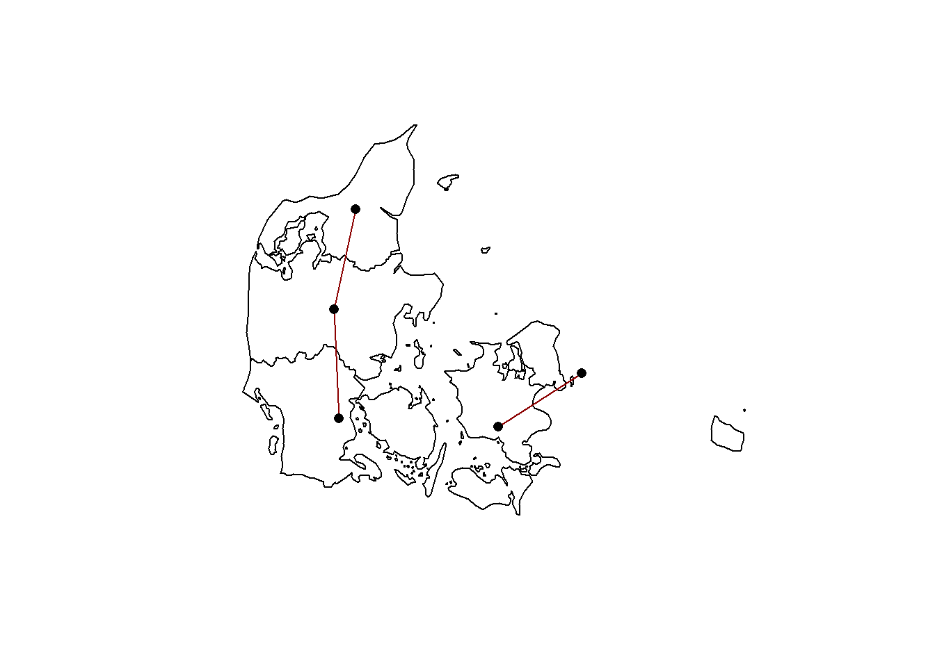
Now we plot the neighborhood weight to see if the Zealand island is linked to Jutland peninsula. The data is in the .nb file. It looks like we may need to recalculate the neighborhood as there are bridges between Zealand and Zealand. This is different situation from Staten Island and the other boroughs of New York.

library(spdep)

#contiguity based neighbourhood
DKnut2.nb<-poly2nb(DKnuts2_sf2) 
DKnut2.nb
Neighbour list object:
Number of regions: 5 
Number of nonzero links: 6 
Percentage nonzero weights: 24 
Average number of links: 1.2 
is.symmetric.nb(DKnut2.nb) 
[1] TRUE

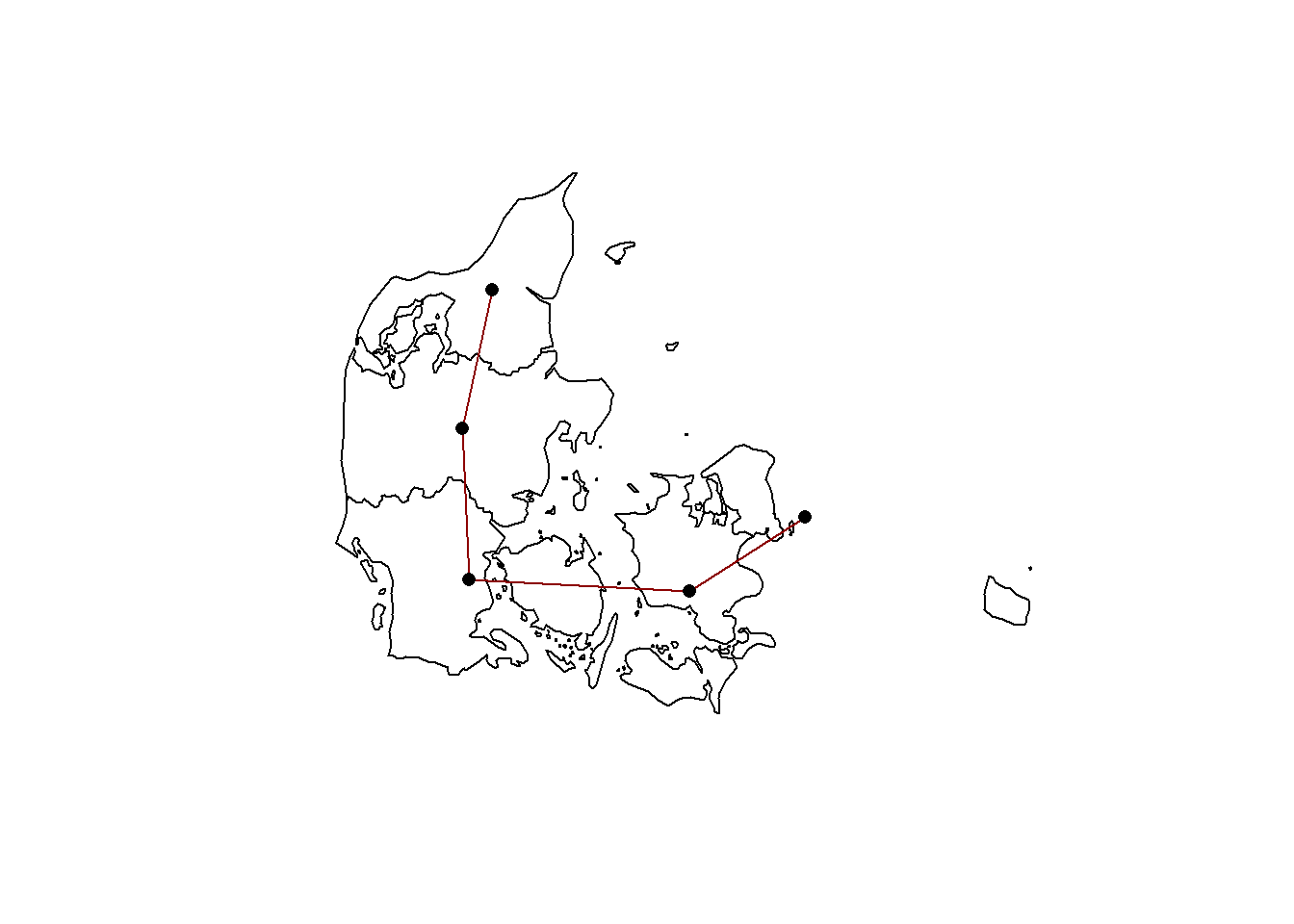
Plotting in base R with sf object requires extracting the geometry and coordinates. Need to modify the link between Zealand and Jutland.

plot(st_geometry(DKnuts2_sf2))
plot(DKnut2.nb,coords=st_coordinates(st_centroid(st_geometry(DKnuts2_sf2))),
     add=TRUE,pch=16,col='darkred')

The solution is provided in stack overflow. https://gis.stackexchange.com/questions/413159/how-to-assign-a-neighbour-status-to-unlinked-polygons

DKconnect <- function(polys, nb, distance="centroid"){
    
    if(distance == "centroid"){
        coords = sf::st_coordinates(sf::st_centroid(sf::st_geometry(polys)))
        dmat = as.matrix(dist(coords))
    }else if(distance == "polygon"){
        dmat = sf::st_distance(polys) + 1 # offset for adjacencies
        diag(dmat) = 0 # no self-intersections
    }else{
        stop("Unknown distance method")
    }
    
    gfull = igraph::graph.adjacency(dmat, weighted=TRUE, mode="undirected")
    gmst = igraph::mst(gfull)
    edgemat = as.matrix(igraph::as_adj(gmst))
    edgelistw = spdep::mat2listw(edgemat)
    edgenb = edgelistw$neighbour
    attr(edgenb,"region.id") = attr(nb, "region.id")
    allnb = spdep::union.nb(nb, edgenb)
    allnb
}

#run function
DKnut2_connected.nb = DKconnect(DKnuts2_sf2,DKnut2.nb)
Warning in spdep::mat2listw(edgemat): style is M (missing); style should be set
to a valid value
plot(st_geometry(DKnuts2_sf2))
plot(DKnut2_connected.nb,
     coords=st_coordinates(st_centroid(st_geometry(DKnuts2_sf2))),
     add=TRUE,pch=16,col='darkred')

#create spatial weights for neighbour lists
r.id<-attr(DKnuts2_sf2,"id")
lw <- nb2listw(DKnut2_connected.nb,zero.policy = TRUE) #W=row standardised

Perform robust regression

#robust linear models
DKnuts2_sf2$resids <- MASS::rlm(SMR~maleper,data=DKnuts2_sf2)$res

#tmap robust linear model-residual
#plot using color blind argument
tm_shape(DKnuts2_sf2) + tm_polygons(col='resids',title='Residuals')+
  tm_style("col_blind")
Variable(s) "resids" contains positive and negative values, so midpoint is set to 0. Set midpoint = NA to show the full spectrum of the color palette.

Check for spatial autocorrelation using Moran I test.

#globaltest spatial autocorrelation using Moran I test from spdep
gm<-moran.test(DKnuts2_sf2$SMR,listw = lw , 
               na.action = na.omit, zero.policy = T)
gm

    Moran I test under randomisation

data:  DKnuts2_sf2$SMR  
weights: lw    

Moran I statistic standard deviate = -0.98413, p-value = 0.8375
alternative hypothesis: greater
sample estimates:
Moran I statistic       Expectation          Variance 
       -0.7354200        -0.2500000         0.2432931 

Local test of autocorrelation

#local test of autocorrelation
lm<-localmoran(DKnuts2_sf2$SMR,
    listw = nb2listw(DKnut2_connected.nb, zero.policy = TRUE, 
          style = "C") , na.action = na.omit, zero.policy = T)
lm
          Ii        E.Ii    Var.Ii       Z.Ii Pr(z != E(Ii))
1 -0.4777173 -0.20238585 0.4276556 -0.4210259      0.6737362
2 -0.9220960 -0.21612919 0.4418446 -1.0620611      0.2882079
3 -1.3492564 -0.49175508 0.6214513 -1.0877554      0.2767031
4 -0.2490245 -0.14095220 0.2605379 -0.2117284      0.8323189
5 -0.1984676 -0.09276265 0.1789140 -0.2499040      0.8026616
attr(,"call")
localmoran(x = DKnuts2_sf2$SMR, listw = nb2listw(DKnut2_connected.nb, 
    zero.policy = TRUE, style = "C"), zero.policy = T, na.action = na.omit)
attr(,"class")
[1] "localmoran" "matrix"     "array"     
attr(,"quadr")
       mean   median    pysal
1  High-Low High-Low High-Low
2   Low-Low  Low-Low Low-High
3 High-High High-Low High-Low
4  Low-High Low-High Low-High
5  Low-High Low-High Low-High

Spatial regression with spdep. The spatial filtering removes spatial dependency for regression analysis.

##spdep & spatialreg
fit.ols<-lm(SMR~maleper, data=DKnuts2_sf2, 
            listw=lw,zero.policy=T, 
            type="lag", method="spam")
Warning in lm(SMR ~ maleper, data = DKnuts2_sf2, listw = lw, zero.policy = T, :
method = 'spam' is not supported. Using 'qr'
Warning: In lm.fit(x, y, offset = offset, singular.ok = singular.ok, ...) :
 extra arguments 'listw', 'zero.policy', 'type' will be disregarded
summary(fit.ols)

Call:
lm(formula = SMR ~ maleper, data = DKnuts2_sf2, method = "spam", 
    listw = lw, zero.policy = T, type = "lag")

Residuals:
       1        2        3        4        5 
 0.03010 -0.01345  0.11401 -0.07059 -0.06007 

Coefficients:
            Estimate Std. Error t value Pr(>|t|)
(Intercept)    5.994      3.980   1.506    0.229
maleper       -2.475      1.984  -1.247    0.301

Residual standard error: 0.08694 on 3 degrees of freedom
Multiple R-squared:  0.3416,    Adjusted R-squared:  0.1221 
F-statistic: 1.556 on 1 and 3 DF,  p-value: 0.3007

SAR - Lag model. The functions from *spdep* have been moved to spatialreg .

library(spatialreg)
fit.lag<-lagsarlm(SMR~maleper, data=DKnuts2_sf2, 
                  listw=lw,zero.policy=T, 
                  type="lag", method="spam")

summary(fit.lag, Nagelkerke=T)

Call:lagsarlm(formula = SMR ~ maleper, data = DKnuts2_sf2, listw = lw, 
    type = "lag", method = "spam", zero.policy = T)

Residuals:
       Min         1Q     Median         3Q        Max 
-0.0443592 -0.0341796  0.0030004  0.0291800  0.0463583 

Type: lag 
Coefficients: (asymptotic standard errors) 
            Estimate Std. Error z value Pr(>|z|)
(Intercept)  3.17355    1.60916  1.9722  0.04859
maleper     -0.66296    0.80039 -0.8283  0.40750

Rho: -0.78891, LR test value: 3.8347, p-value: 0.050202
Asymptotic standard error: 0.15282
    z-value: -5.1625, p-value: 2.4366e-07
Wald statistic: 26.652, p-value: 2.4366e-07

Log likelihood: 8.312303 for lag model
ML residual variance (sigma squared): 0.0012291, (sigma: 0.035059)
Nagelkerke pseudo-R-squared: 0.6942 
Number of observations: 5 
Number of parameters estimated: 4 
AIC: -8.6246, (AIC for lm: -6.7899)
LM test for residual autocorrelation
test value: 1.3631, p-value: 0.24301

Spatial Durbin Model

#spatialreg

fit.durb<-lagsarlm(SMR~maleper,data=DKnuts2_sf2, 
                   listw=lw,zero.policy=T, type="mixed", 
                   method="spam")

summary(fit.durb, Nagelkerke=T)

Call:lagsarlm(formula = SMR ~ maleper, data = DKnuts2_sf2, listw = lw, 
    type = "mixed", method = "spam", zero.policy = T)

Residuals:
       Min         1Q     Median         3Q        Max 
-0.0437252  0.0012719  0.0059890  0.0111566  0.0253077 

Type: mixed 
Coefficients: (asymptotic standard errors) 
            Estimate Std. Error z value Pr(>|z|)
(Intercept) -2.00246    2.17036 -0.9226  0.35620
maleper     -1.83172    0.89172 -2.0541  0.03996
lag.maleper  3.68229    1.43910  2.5587  0.01050

Rho: -0.65582, LR test value: 2.5041, p-value: 0.11355
Asymptotic standard error: 0.22276
    z-value: -2.9441, p-value: 0.0032394
Wald statistic: 8.6675, p-value: 0.0032394

Log likelihood: 10.89748 for mixed model
ML residual variance (sigma squared): 0.00054287, (sigma: 0.023299)
Nagelkerke pseudo-R-squared: 0.89127 
Number of observations: 5 
Number of parameters estimated: 5 
AIC: -11.795, (AIC for lm: -11.291)
LM test for residual autocorrelation
test value: 0.080005, p-value: 0.77729

Spatial Durbin Error Model

fit.errdurb<-errorsarlm(SMR~maleper, 
        data=DKnuts2_sf2, 
        listw=lw,zero.policy=T,etype="emixed", method="spam")

summary(fit.errdurb, Nagelkerke=T)

Call:errorsarlm(formula = SMR ~ maleper, data = DKnuts2_sf2, listw = lw, 
    etype = "emixed", method = "spam", zero.policy = T)

Residuals:
       Min         1Q     Median         3Q        Max 
-0.0607695  0.0033715  0.0101663  0.0167347  0.0304970 

Type: error 
Coefficients: (asymptotic standard errors) 
            Estimate Std. Error z value  Pr(>|z|)
(Intercept)  -3.4224     2.4849 -1.3773 0.1684182
maleper      -3.7461     1.0337 -3.6238 0.0002903
lag.maleper   5.9680     1.8468  3.2316 0.0012311

Lambda: -0.36381, LR test value: 0.6199, p-value: 0.43109
Asymptotic standard error: 0.34301
    z-value: -1.0606, p-value: 0.28886
Wald statistic: 1.1249, p-value: 0.28886

Log likelihood: 9.955379 for error model
ML residual variance (sigma squared): 0.0010036, (sigma: 0.031679)
Nagelkerke pseudo-R-squared: 0.84151 
Number of observations: 5 
Number of parameters estimated: 5 
AIC: NA (not available for weighted model), (AIC for lm: -11.291)

SAC Model

fit.sac<-sacsarlm(SMR~maleper,
                  data=DKnuts2_sf2, 
                  listw=lw,zero.policy=T, 
                  type="sac", method="MC")

summary(fit.sac, Nagelkerke=T)

Call:sacsarlm(formula = SMR ~ maleper, data = DKnuts2_sf2, listw = lw, 
    type = "sac", method = "MC", zero.policy = T)

Residuals:
      Min        1Q    Median        3Q       Max 
-0.034569 -0.028384 -0.004774  0.033291  0.034436 

Type: sac 
Coefficients: (numerical Hessian approximate standard errors) 
            Estimate Std. Error z value Pr(>|z|)
(Intercept) 1.475165   1.583042  0.9319   0.3514
maleper     0.099753   0.817024  0.1221   0.9028

Rho: -0.62625
Approximate (numerical Hessian) standard error: 0.31056
    z-value: -2.0165, p-value: 0.043744
Lambda: -0.60661
Approximate (numerical Hessian) standard error: 0.41076
    z-value: -1.4768, p-value: 0.13973

LR test value: 3.9764, p-value: 0.13694

Log likelihood: 8.383149 for sac model
ML residual variance (sigma squared): 0.00086351, (sigma: 0.029386)
Nagelkerke pseudo-R-squared: 0.70274 
Number of observations: 5 
Number of parameters estimated: 5 
AIC: -6.7663, (AIC for lm: -6.7899)

spatial filtering

#function from spatialreg
#Set ExactEV=TRUE to use exact expectations and variances rather than the expectation and variance of Moran's I from the previous iteration, default FALSE

DKFilt<-SpatialFiltering(SMR~maleper, 
        data=DKnuts2_sf2,
        nb=DKnut2_connected.nb,
        #ExactEV = TRUE,
        zero.policy = TRUE,style="W")
   An inversion has been detected. The procedure will terminate now.
   It is suggested to use the exact expectation and variance of Moran's I
   by setting the option ExactEV to TRUE.

14.4.3 INLA

This section uses Bayesian modeling for regression with fitting of the model by Integrated Nested Lapace Approximation (INLA). https://www.r-bloggers.com/spatial-data-analysis-with-inla/. For those wanting to analyse leukemia in New York instead of COVID-19, the dataset NY8 is available from DClusterm. INLA approximates the posterior distribution as latent Gaussian Markov random field. In this baseline analysis, the poisson model is performed without any random effect terms.

library(INLA)

nb2INLA("DKnut2.graph", DKnut2_connected.nb)
#This create a file called ``LDN-INLA.adj'' with the graph for INLA

DK.adj <- paste(getwd(),"/DK.graph",sep="")

#Poisson model with no random latent effect-ideal baseline model
m1<-inla(SMR~ 1+maleper, data=DKnuts2_sf2, 
         family="poisson",
         E=DKnuts2_sf2$Expected,
         control.predictor = list(compute = TRUE),
         control.compute = list(dic = TRUE, waic = TRUE), 
         verbose = T )

R1<-summary(m1)

In this next analysis, the Poisson model was repeated with random effect terms. This step was facilitated by adding the index term.

#Poisson model with random effect 
#index to identify random effect ID
DKnuts2_sf2$ID <- 1:nrow(DKnuts2_sf2)
m2<-inla(SMR~ 1+ maleper +f(ID, model = "iid"), 
         data=DKnuts2_sf2, family="poisson",
         E=DKnuts2_sf2$Expected,
         control.predictor = list(compute = TRUE),
         control.compute = list(dic = TRUE, waic = TRUE))

R2<-summary(m2)

Plot SMR

DKnut2_sf2$FIXED.EFF <- m1$summary.fitted[, "mean"]
DKnut2_sf2$IID.EFF <- m2$summary.fitted[, "mean"]

#plot regression on map
tSMR<-tm_shape(DKnuts2_sf2)+tm_polygons("SMR")

Plot the fixed model.

tFIXED<-tm_shape(DKnuts2_sf2)+tm_polygons("FIXED.EFF")

Plot the IID model.

tIID<-tm_shape(DKnuts2_sf2)+tm_polygons("IID.EFF")

This next paragraph involves the use of spatial random effects in regression models. Examples include conditional autoregressive (CAR) and intrinsic CAR (ICAR).

# Create sparse adjacency matrix
DK.mat <- as(nb2mat(DKnut2_connected.nb, 
                    style = "B",zero.policy = TRUE),"Matrix") 

#S=variance stabilise
# Fit model
m.icar <- inla(SMR ~ 1+maleper+   
    f(ID, model = "besag", graph = DK.mat),
  data = DKnuts2_sf2, E = DKnuts2_sf2$Expected, family ="poisson",
  control.predictor = list(compute = TRUE),
  control.compute = list(dic = TRUE, waic = TRUE))

R3<-summary(m.icar)

The Besag-York-Mollie (BYM) now accounts for spatial dependency of neighbours. It includes random effect from ICA and index.

m.bym = inla(SMR ~ -1+ maleper+   
    f(ID, model = "bym", graph = DK.mat),
  data = DKnuts2_sf2, E = DKnuts2_sf2$Expected, family ="poisson",
  control.predictor = list(compute = TRUE),
  control.compute = list(dic = TRUE, waic = TRUE))

R4<-summary(m.bym)
ICARmatrix <- Diagonal(nrow(DK.mat), apply(DK.mat, 1, sum)) - DK.mat
Cmatrix <- Diagonal(nrow(DKnuts2_sf2), 1) -  ICARmatrix
max(eigen(Cmatrix)$values)
m.ler = inla(SMR ~ -1+maleper+ 
    f(ID, model = "generic1", Cmatrix = Cmatrix),
  data = DKnuts2_sf2, E = DKnuts2_sf2$Expected, family ="poisson",
  control.predictor = list(compute = TRUE),
  control.compute = list(dic = TRUE, waic = TRUE))
R5<-summary(m.ler)

Spatial econometric model such as spatial lag model includes covariates and autoregress on the response variable.

#X
mmatrix <- model.matrix(SMR ~ 1, DKnuts2_sf2)
#W
W <- as(nb2mat(DKnut2_connected.nb, style = "W", zero.policy = TRUE), "Matrix")
#Q
Q.beta = Diagonal(n = ncol(mmatrix), x = 0.001)
#Range of rho
rho.min<- -1
rho.max<- 1
#Arguments for 'slm'
args.slm = list(
   rho.min = rho.min ,
   rho.max = rho.max,
   W = W,
   X = mmatrix,
   Q.beta = Q.beta
)
#Prior on rho
hyper.slm = list(
   prec = list(
      prior = "loggamma", param = c(0.01, 0.01)),
      rho = list(initial=0, prior = "logitbeta", param = c(1,1))
)

#SLM model
m.slm <- inla( SMR ~ -1+maleper+
     f(ID, model = "slm", args.slm = args.slm, hyper = hyper.slm),
   data = DKnuts2_sf2, family = "poisson",
   E = DKnuts2_sf2$Expected,
   control.predictor = list(compute = TRUE),
   control.compute = list(dic = TRUE, waic = TRUE)
)

R6<-summary(m.slm)
marg.rho.internal <- m.slm$marginals.hyperpar[["Rho for ID"]]
marg.rho <- inla.tmarginal( function(x) {
  rho.min + x * (rho.max - rho.min)
}, marg.rho.internal)
inla.zmarginal(marg.rho, FALSE)
plot(marg.rho, type = "l", main = "Spatial autocorrelation")

Spatial model selection

DKnut2_sf2$ICAR <- m.icar$summary.fitted.values[, "mean"]
DKnut2_sf2$BYM <- m.bym$summary.fitted.values[, "mean"]
DKnut2_sf2$LEROUX <- m.ler$summary.fitted.values[, "mean"]
DKnut2_sf2$SLM <- m.slm$summary.fitted.values[, "mean"]

labels<-c("Fixed","IID", "ICAR","BYM","LEROUX","SLM")
Marginal_Likelihood<-c(R1$mlik[1],R2$mlik[1],R3$mlik[1],R4$mlik[1],R5$mlik[1],
                       R6$mlik[1])
Marginal_Likelihood<-round(Marginal_Likelihood,2)
WAIC<-c(R1$waic[[1]],R2$waic[[1]],R3$waic[[1]],R4$waic[[1]],R5$waic[[1]],
        R6$waic[[1]])
WAIC<-round(WAIC,2)
DIC<-c(R1$dic[[1]],R2$dic[[1]],R3$dic[[1]],R4$dic[[1]],R5$dic[[1]],R6$dic[[1]])
DIC<-round(DIC,2)
Results<-data.frame(labels,Marginal_Likelihood,WAIC,DIC)
knitr::kable(Results)

#plot maps
tICAR<-tm_shape(DKnut2_sf2)+tm_polygons("ICAR")
tBYM<-tm_shape(DKnut2_sf2)+tm_polygons("BYM")
tLEROUX<-tm_shape(DKnut2_sf2)+tm_polygons("LEROUX")
tSLM<-tm_shape(DKnut2_sf2)+tm_polygons("SLM")
#arrange in grid using tmap arrange
current.mode <- tmap_mode("plot")
tmap_arrange(tFIXED,tIID,tICAR,tBYM,tLEROUX,tSLM)
tmap_mode(current.mode)

14.4.4 Stan

library(brms)
Warning: package 'brms' was built under R version 4.3.3
Loading required package: Rcpp
Loading 'brms' package (version 2.22.0). Useful instructions
can be found by typing help('brms'). A more detailed introduction
to the package is available through vignette('brms_overview').

Attaching package: 'brms'
The following object is masked from 'package:dismo':

    kfold
The following object is masked from 'package:stats':

    ar
#S=variance stabilise
# Fit model

#brm.lag<- brm (COVIDdeathraw ~ 1+Age65raw+Income+sar(NY.nb, type = "lag"),
#               data = DKnut2_sf2, data2 = list(NY.nb = NY.nb),
#            chains = 2, cores = 2)

14.5 Machine learning in spatial analysis

Up until now we have used frequentist and Bayesian spatial regression methods. Spatial data can also be analysed using machine learning such as random forest and xgboost. XGBoost estimates similar spatial effects as those in SLM and MGWR models.

library(xgboost)

Attaching package: 'xgboost'
The following object is masked from 'package:dplyr':

    slice
library(tidyverse)
library(shapviz)
Warning: package 'shapviz' was built under R version 4.3.3
miami <- miami |>
  transform(
    log_living = log(TOT_LVG_AREA),
    log_land = log(LND_SQFOOT),
    log_price = log(SALE_PRC)
  )

x_coord <- c("LATITUDE", "LONGITUDE")
x_nongeo <- c("log_living", "log_land", "structure_quality", "age")
xvars <- c(x_coord, x_nongeo)

# Select training data
set.seed(1)
ix <- sample(nrow(miami), 0.8 * nrow(miami))
train <- miami[ix, ]
X_train <- train[xvars]
y_train <- train$log_price

# Fit XGBoost model
params <- list(learning_rate = 0.2, nthread = 1)
dtrain <- xgb.DMatrix(data.matrix(X_train), label = y_train, nthread = 1)
fit <- xgb.train(params, dtrain, nrounds = 200)

14.6 Spatio-temporal regression

Spatio-temporal regression combines a spatial model with a temporal model. In many cases of low disease incidence in each region it may not be possible to identify any temporal trend at a regional level.