This section deals with handling of text data. R has several excellent libraries such as tm, tidytext, textmineR and quanteda for handling text data.
In the Data-Wrangling chapter, we had introduced a section on regular expressions. Much of the work is involved in cleaning documents so that unnecessary words such as stop words and white space are removed. Example of stop words include “I”, “he”, “she”, “they” etc. It is also important to turn words into lower case otherwise “London” and “london” are treated as 2 different words.
12.1 Bag of words
Bag of words or unigram analysis describe data in which words in a sentence were separated or tokenised. Later we will demontrate analysis of bigram. Within this bag of words the order of words within the document is not retained. Depending on how this process is performed the negative connotation may be loss. Consider “not green” and after cleaning of the document, only the color “green” remain.
12.2 Extracting data from Pubmed
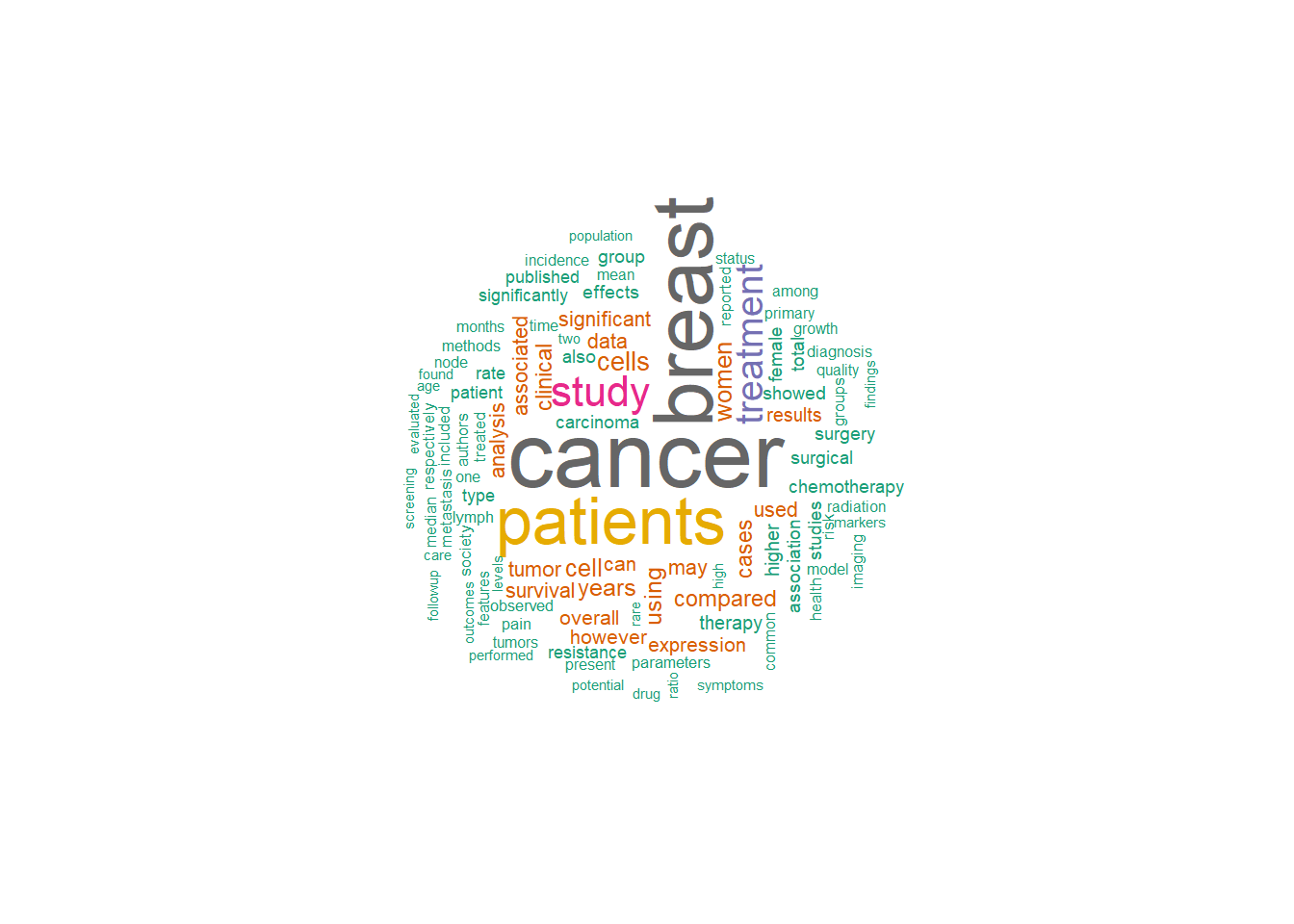
Data can be extracted directly from Pubmed.
library(PubMedWordcloud)#can only extract one word at a time, limit 100 abstractspmid =getPMIDsByKeyWords(keys ="breast cancer", dFrom =2021, dTo =2021, n=100)pmid1 =getPMIDsByKeyWords(keys ="stroke", dFrom =2021, dTo =2021,n=100)#combine 2 search wordsabstracts =getAbstracts(c(pmid,pmid1))
There are total 200 PMIDs
downloading abstracts for PMIDs from 1 to 100 ...
downloading abstracts for PMIDs from 101 to 200 ...
The following objects are masked from 'package:stats':

    filter, lag
The following objects are masked from 'package:base':

    intersect, setdiff, setequal, union
library(SnowballC)library(wordcloud)
Loading required package: RColorBrewer
library(lattice)library(tm)
Loading required package: NLP
Attaching package: 'NLP'
The following object is masked from 'package:ggplot2':

    annotate
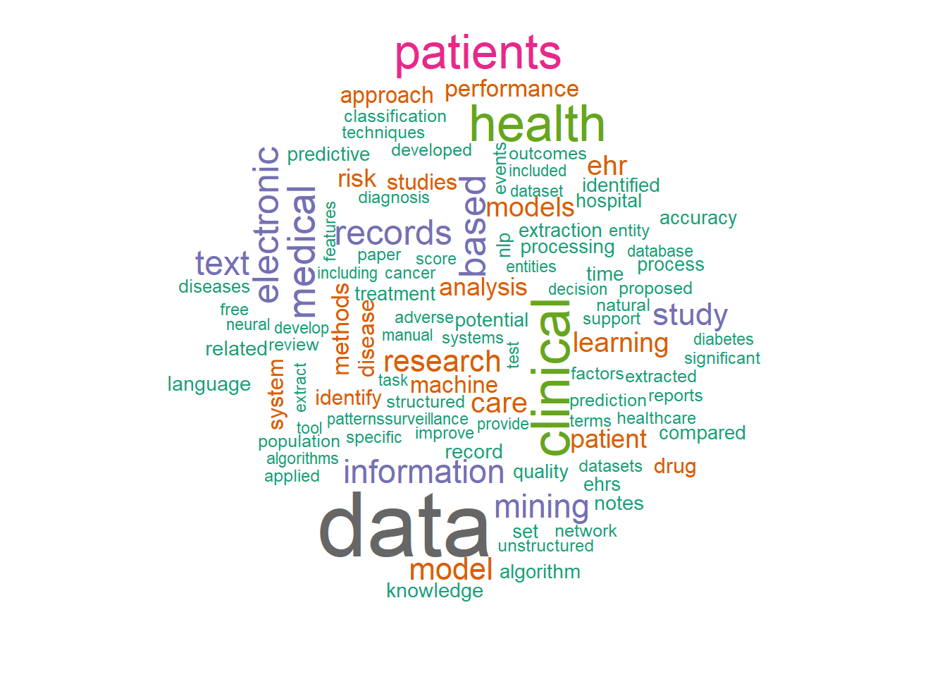
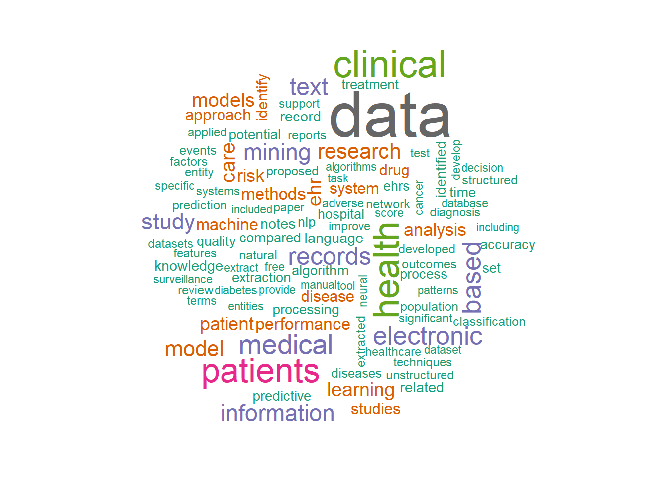
library (dplyr)library(tidytext)library(tidyr)library(stringr)#search 25/9/21#query<-"electronic medical record + text mining"#ngs_search <- EUtilsSummary(query, type="esearch",db = "pubmed",mindate=2016, maxdate=2018, retmax=30000)#summary(ngs_search)#QueryCount(ngs_search)#ngs_records <- EUtilsGet(ngs_search)#save(ngs_records,file="ngs_records.Rda")#bug in system and EUtilsSummary is not working#ISOAbbreviation#reload saved searchload("EMR_Textmiing_ngs_records.Rda")
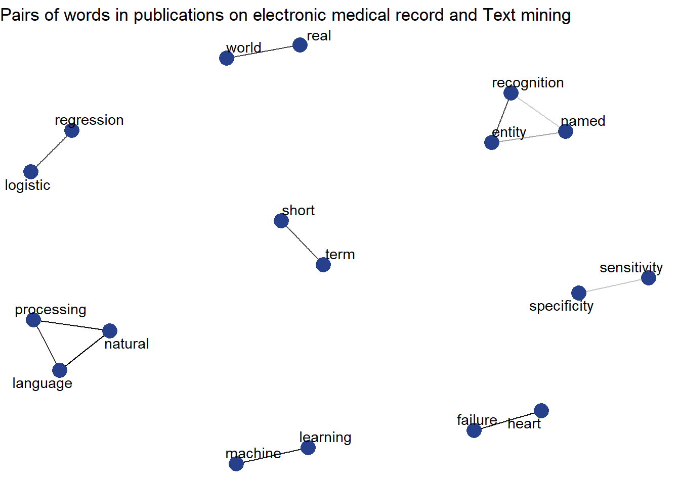
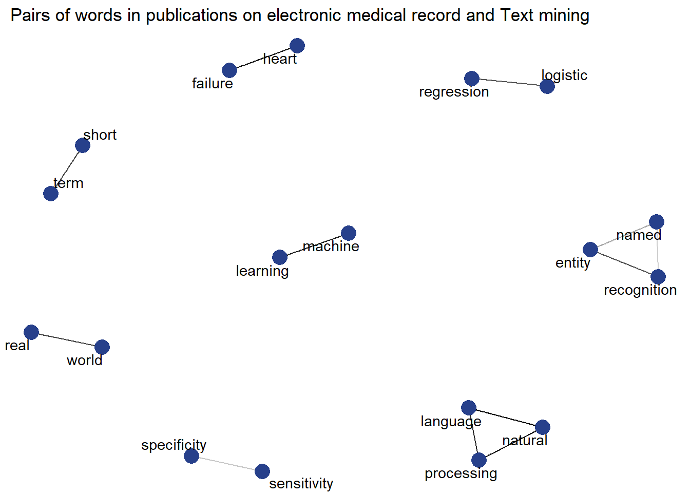
ab_word_cors %>%filter(correlation > .5) %>%graph_from_data_frame() %>%ggraph(layout ="fr") +geom_edge_link(aes(edge_alpha = correlation), show.legend =FALSE) +geom_node_point(color ="#27408b", size =5) +geom_node_text(aes(label = name), repel =TRUE) +theme_void(base_family="Roboto")+labs(title="Pairs of words in publications on electronic medical record and Text mining ")
graph analysis of word relationship
library(extrafont)library(igraph)library(ggraph)library(widyr)library(viridis)#abstractab_word_cors <- ab_word %>%mutate(section =row_number() %/%10) %>%filter(section >0) %>%filter(!word %in% stop_words$word) %>%group_by(word) %>%filter(n() >=20) %>%pairwise_cor(word, section, sort =TRUE)ab_word_cors %>%filter(correlation > .5) %>%graph_from_data_frame() %>%ggraph(layout ="fr") +geom_edge_link(aes(edge_alpha = correlation), show.legend =FALSE) +geom_node_point(color ="#27408b", size =5) +geom_node_text(aes(label = name), repel =TRUE) +theme_void(base_family="Roboto")+labs(title=" Pairs of words in publications on electronic medical record and Text mining ")
12.3 Bigram analysis
Previously we treated words as unigram. Here we group words which appear together as bigram.
ab_bigrams <- ab %>%unnest_tokens(bigram, text, token ="ngrams", n =2) %>%mutate(bigram =gsub("[^A-Za-z ]","", bigram)) %>%filter(bigram !="")
Warning: Outer names are only allowed for unnamed scalar atomic inputs
# A tibble: 21,793 × 8
   author datetimestamp       description heading id    language origin bigram
   <lgl>  <dttm>              <lgl>       <lgl>   <chr> <chr>    <lgl>  <chr>
 1 NA     2025-02-11 02:43:08 NA          NA      1     en       NA     growing…
 2 NA     2025-02-11 02:43:08 NA          NA      1     en       NA     elderly…
 3 NA     2025-02-11 02:43:08 NA          NA      1     en       NA     populat…
 4 NA     2025-02-11 02:43:08 NA          NA      1     en       NA     incurab…
 5 NA     2025-02-11 02:43:08 NA          NA      1     en       NA     chronic…
 6 NA     2025-02-11 02:43:08 NA          NA      1     en       NA     continu…
 7 NA     2025-02-11 02:43:08 NA          NA      1     en       NA     medical…
 8 NA     2025-02-11 02:43:08 NA          NA      1     en       NA     service…
 9 NA     2025-02-11 02:43:08 NA          NA      1     en       NA     mental …
10 NA     2025-02-11 02:43:08 NA          NA      1     en       NA     impairm…
# ℹ 21,783 more rows
IGRAPH f45d754 DN-- 107 97 --
+ attr: name (v/c), n (e/n)
+ edges from f45d754 (vertex names):
 [1]           ->            electronic->health      machine   ->learning
 [4] health    ->records     text      ->mining      data      ->mining
 [7] natural   ->language    language  ->processing  medical   ->records
[10]           ->patients    electronic->medical     health    ->care
[13] ehr       ->data        health    ->record      free      ->text
[16] clinical  ->notes       deep      ->learning    clinical  ->data
[19] entity    ->recognition medical   ->record      processing->nlp
[22] neural    ->network     records   ->ehrs        logistic  ->regression
+ ... omitted several edges
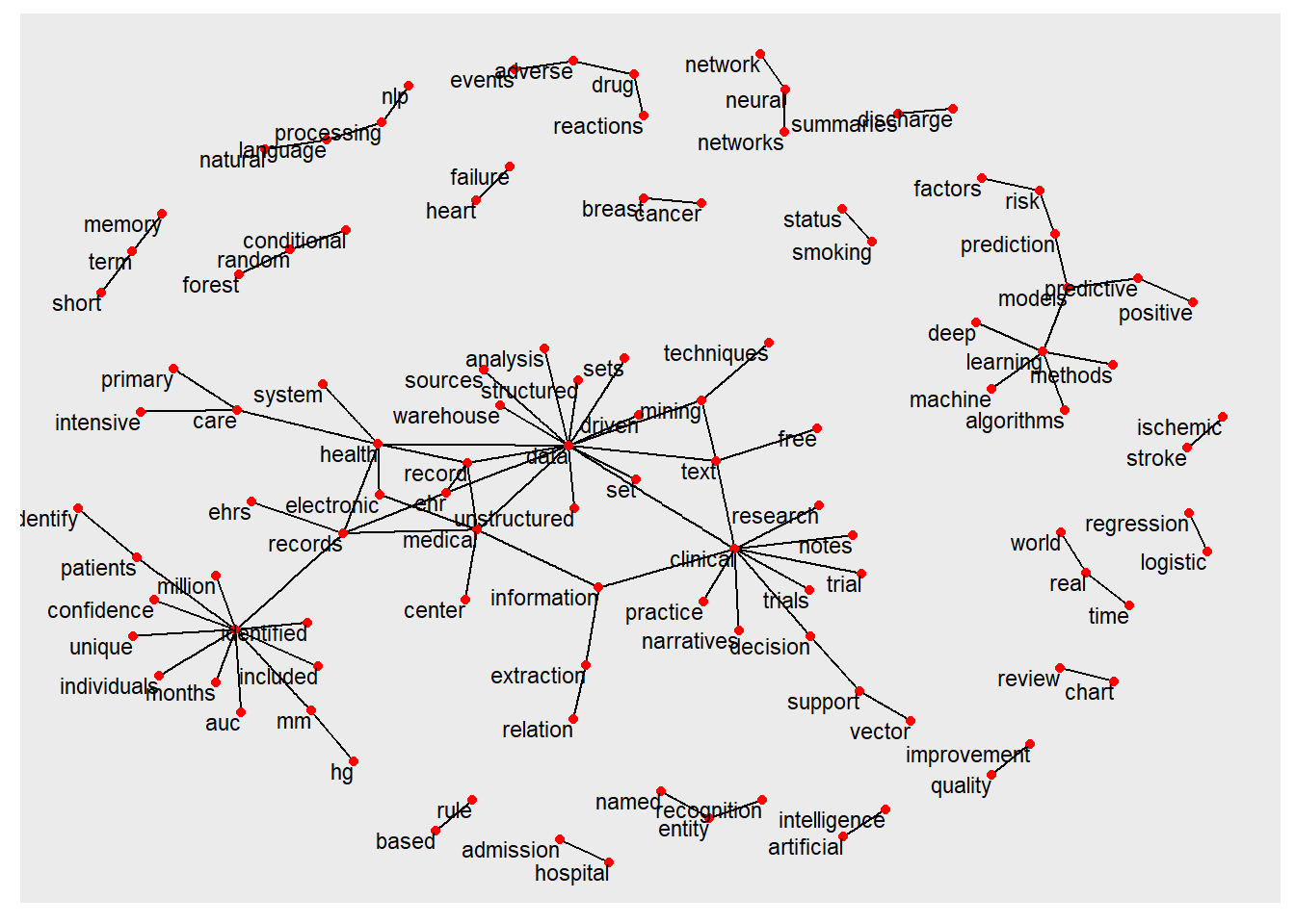
12.3.1 Network of bigrams
The relationship among the bigrams are illustrated here.
library(tidygraph)
Attaching package: 'tidygraph'
The following object is masked from 'package:igraph':

    groups
The following object is masked from 'package:stats':

    filter
as_tbl_graph(bigram_graph)
# A tbl_graph: 107 nodes and 97 edges
#
# A directed multigraph with 20 components
#
# A tibble: 107 × 1
  name
  <chr>
1 ""
2 "electronic"
3 "machine"
4 "health"
5 "text"
6 "data"
# ℹ 101 more rows
#
# A tibble: 97 × 3
   from    to     n
  <int> <int> <int>
1     1     1   533
2     2     4   173
3     3    27   119
# ℹ 94 more rows
# A tibble: 21,793 × 8
   author datetimestamp       description heading id    language origin trigram
   <lgl>  <dttm>              <lgl>       <lgl>   <chr> <chr>    <lgl>  <chr>
 1 NA     2025-02-11 02:43:08 NA          NA      1     en       NA     growing…
 2 NA     2025-02-11 02:43:08 NA          NA      1     en       NA     elderly…
 3 NA     2025-02-11 02:43:08 NA          NA      1     en       NA     populat…
 4 NA     2025-02-11 02:43:08 NA          NA      1     en       NA     incurab…
 5 NA     2025-02-11 02:43:08 NA          NA      1     en       NA     chronic…
 6 NA     2025-02-11 02:43:08 NA          NA      1     en       NA     continu…
 7 NA     2025-02-11 02:43:08 NA          NA      1     en       NA     medical…
 8 NA     2025-02-11 02:43:08 NA          NA      1     en       NA     service…
 9 NA     2025-02-11 02:43:08 NA          NA      1     en       NA     mental …
10 NA     2025-02-11 02:43:08 NA          NA      1     en       NA     impairm…
# ℹ 21,783 more rows
Two methods for unsupervised thematic analysis, NMF and probabilistic topic model, are illustrated.
12.5.1 TFIDF
Term frequency defines the frequency of a term in a document. The document frequency defines how often a term is used across document. The inverse document frequency can be seen as a weight to decrease the importance of commonly words used across documents. Term frequency inverse document frequency is a process used to down weight common terms and highlight important terms in the document. In the example below topic modeling, an example of creating tfidf is shown. Other packages like tidytext, textmineR have functions for creating tfidf
library(slam)library(topicmodels)ab2<-ab %>%select(text) %>%as.data.frame()corpus =Corpus(VectorSource(ab2))myCorpus =VCorpus(VectorSource(ab2))myCorpus <-tm_map(myCorpus, content_transformer(tolower))myCorpus <-tm_map(myCorpus, removeNumbers)myCorpus <-tm_map(myCorpus, removePunctuation)myCorpus <-tm_map(myCorpus, removeWords, stopwords ("english"),lazy=TRUE) myCorpus <-tm_map(myCorpus, stripWhitespace, lazy=TRUE)# create term-document matrixdtm <-DocumentTermMatrix(myCorpus,control =list(wordLengths=c(3, 20)))tdm <-TermDocumentMatrix(myCorpus,control =list(wordLengths=c(3, 20)))#convert to matrixtdm =as.matrix(tdm)#ensure non non zero entryrowTotals <-apply(dtm , 1, sum) #Find the sum of words in each Documentdtm1 <- dtm[rowTotals>0, ] #create tfidf using slam libraryterm_tfidf <-+tapply(dtm$v/row_sums(dtm)[dtm$i],dtm$j,mean) *+log2(nDocs(dtm)/col_sums(dtm>0))#remove frequent wordsdtm1 <-dtm1[,term_tfidf>=median(term_tfidf)] #dtm <-dtm[,term_tfidf>=0.0015]
12.5.2 Latent Dirichlet Allocation
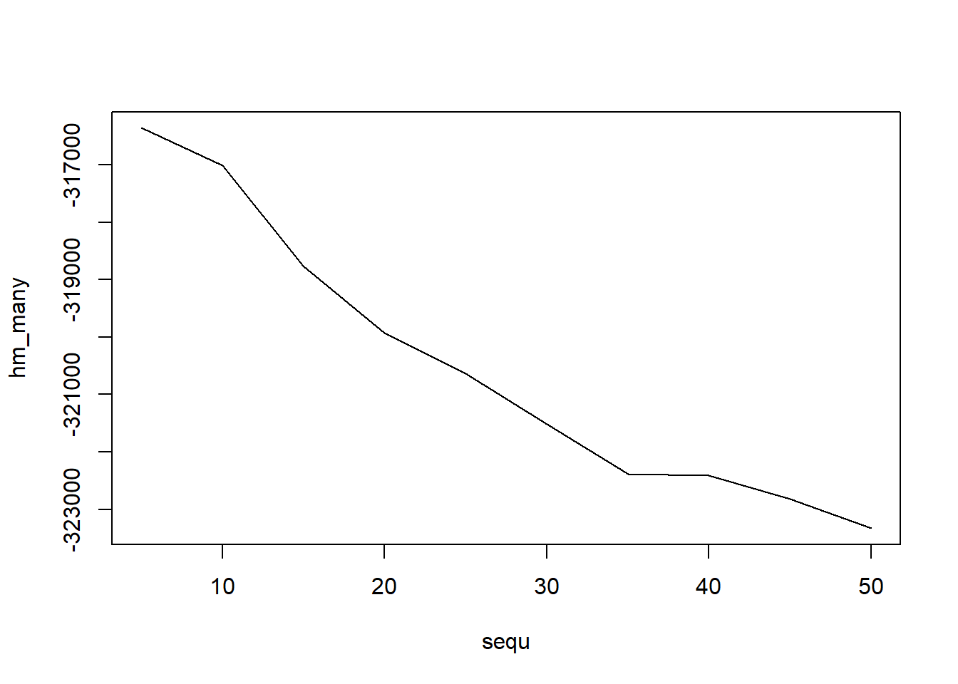
Probabilistic topic modelling is a machine learning method that generates topics or discovers themes among a collection of documents. This step was performed using the Latent Dirichlet Allocation algorithm via the topicmodels package in R. An issue with topic modeling is that the number of topics are not known. It can be estimated empirically or by examining the harmonic means of the log likelihood . The idea is that the number of topics based on the log likelihood of P(topics|documents) at each iterations
Determine the optimal number of topics based on harmonic means.
## estimate kk =20burnin =1000iter =1000keep=50fitted <-LDA(dtm1, k = k, method ="Gibbs",control =list(burnin = burnin, iter = iter, keep = keep) )# where keep indicates that every keep iteration the log-likelihood is evaluated and stored. This returns all log-likelihood values including burnin, i.e., these need to be omitted before calculating the harmonic mean:logLiks <- fitted@logLiks[-c(1:(burnin/keep))]# assuming that burnin is a multiple of keep andharmonicMean(logLiks)
Loading required package: gmp
Attaching package: 'gmp'
The following objects are masked from 'package:base':

    %*%, apply, crossprod, matrix, tcrossprod
C code of R package 'Rmpfr': GMP using 64 bits per limb
Attaching package: 'Rmpfr'
The following object is masked from 'package:gmp':

    outer
The following objects are masked from 'package:stats':

    dbinom, dgamma, dnbinom, dnorm, dpois, dt, pnorm
The following objects are masked from 'package:base':

    cbind, pmax, pmin, rbind
[1] -320584.7
# generate numerous topic models with different numbers of topicssequ <-seq(5, 50, 5) # in this case a sequence of numbers from 5 to 50, by 5.fitted_many <-lapply(sequ, function(k) LDA(dtm1, k = k, method ="Gibbs",control =list(burnin = burnin, iter = iter, keep = keep) ))# extract logliks from each topiclogLiks_many <-lapply(fitted_many, function(L) L@logLiks[-c(1:(burnin/keep))])# compute harmonic meanshm_many <-sapply(logLiks_many, function(h) harmonicMean(h))# inspectplot(sequ, hm_many, type ="l")
# compute optimum number of topicssequ[which.max(hm_many)]
[1] 5
The previous analysis show that there are 40 topics. For ease of illustrations LDA is perform with 5 topics.
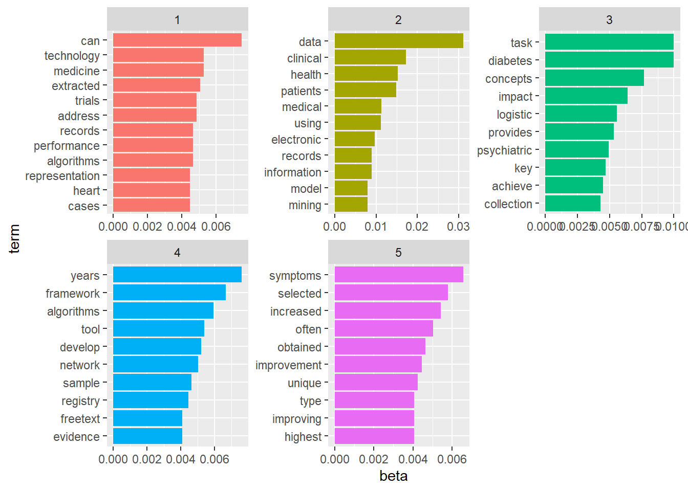
#perform LDAlda_EHR <-LDA(dtm1, k = sequ[which.max(hm_many)], method="Gibbs", control=list(seed=1234,burnin=1000,thin=100,iter=1000))#extract topics terms and beta weightsEHR_topics <-tidy(lda_EHR, matrix ="beta")#view data by topicsEHR_top_terms <- EHR_topics %>%group_by(topic) %>%slice_max(beta, n =10) %>%ungroup() %>%arrange(topic, -beta)EHR_top_terms %>%mutate(term =reorder_within(term, beta, topic)) %>%ggplot(aes(beta, term, fill =factor(topic))) +geom_col(show.legend =FALSE) +facet_wrap(~ topic, scales ="free") +scale_y_reordered()
In the previous chapter, NMF was used as a method to cluster data. Here, it can be framed as a method for topic modeling. NMF is analogous to multinomial PCA or probabilistic latent semantic analysis.
library(NMF)
Warning: package 'NMF' was built under R version 4.3.2
The following objects are masked from 'package:igraph':

    algorithm, compare
res <-nmf(as.matrix(tdm), sequ[which.max(hm_many)], "lee")
Warning in validityMethod(object): Dimensions of W and H look strange [ncol(W)=
5 > ncol(H)= 1 ]
Warning in validityMethod(object): Dimensions of W and H look strange [ncol(W)=
5 > ncol(H)= 1 ]

Warning in validityMethod(object): Dimensions of W and H look strange [ncol(W)=
5 > ncol(H)= 1 ]
                  Topic1       Topic2       Topic3       Topic4      Topic5
data        0.0159593720 0.0282241995 0.0100832967 0.0261308474 0.009280678
health      0.0009194075 0.0181108217 0.0043249907 0.0200148184 0.003487443
clinical    0.0112117568 0.0017558221 0.0179071444 0.0119635890 0.001939906
records     0.0062592077 0.0068971277 0.0004992859 0.0116797218 0.015787157
patients    0.0135102987 0.0172660375 0.0015100847 0.0038115459 0.001999944
medical     0.0087560848 0.0036455271 0.0118192185 0.0005089656 0.009446978
using       0.0002018923 0.0073490332 0.0127421083 0.0062441034 0.007323748
electronic  0.0107998221 0.0004045812 0.0076442762 0.0063438294 0.005712474
model       0.0005598215 0.0010319464 0.0055814410 0.0153828778 0.008074580
information 0.0036473004 0.0061528286 0.0052446082 0.0074690427 0.006044581
                 total        word
data        0.08967839        data
health      0.04685748      health
clinical    0.04477822    clinical
records     0.04112250     records
patients    0.03809791    patients
medical     0.03417677     medical
using       0.03386089       using
electronic  0.03090498  electronic
model       0.03063067       model
information 0.02855836 information
                Topic1       Topic2      Topic3       Topic4      Topic5
data       0.015959372 0.0282241995 0.010083297 0.0261308474 0.009280678
patients   0.013510299 0.0172660375 0.001510085 0.0038115459 0.001999944
clinical   0.011211757 0.0017558221 0.017907144 0.0119635890 0.001939906
electronic 0.010799822 0.0004045812 0.007644276 0.0063438294 0.005712474
medical    0.008756085 0.0036455271 0.011819218 0.0005089656 0.009446978
based      0.006544277 0.0001106726 0.001261345 0.0035722560 0.007048943
                 word
data             data
patients     patients
clinical     clinical
electronic electronic
medical       medical
based           based
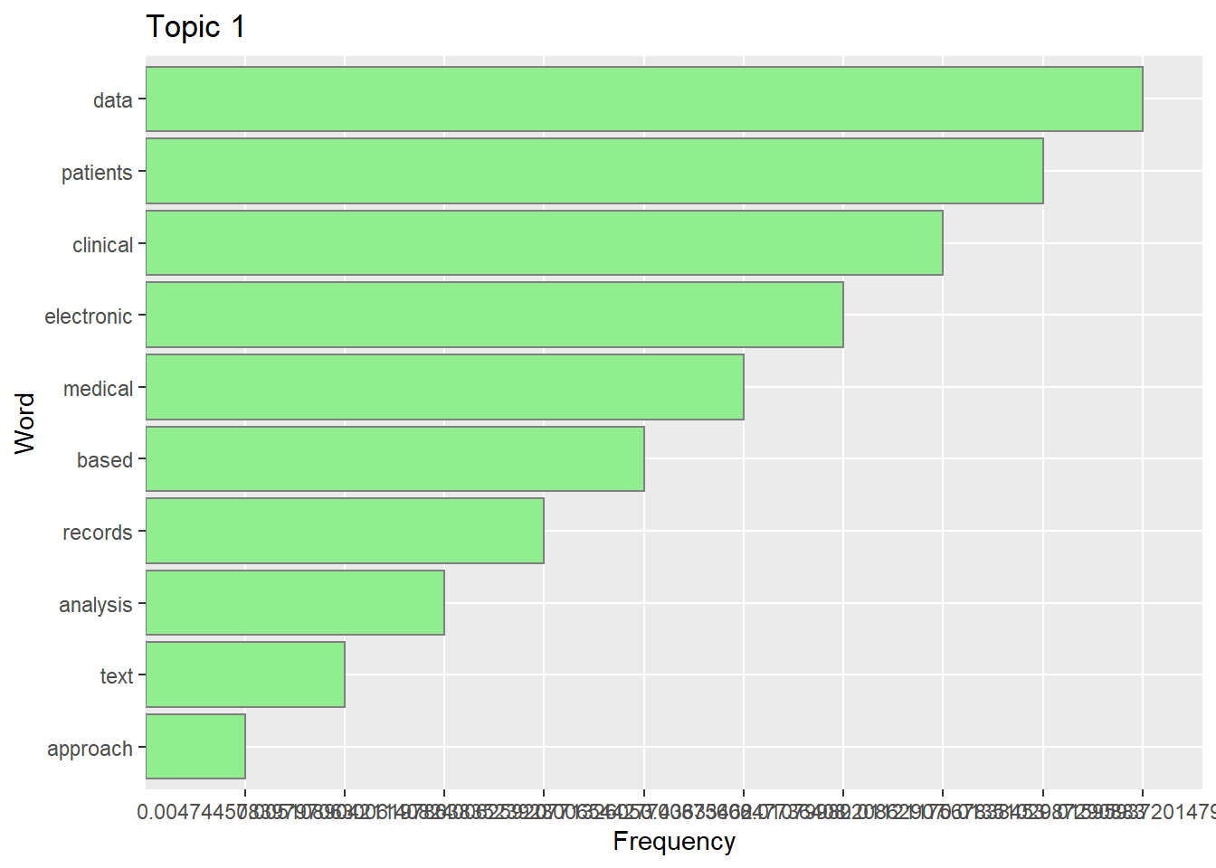
Plot topic 1
d <- newdatadf <-as.data.frame(cbind(d[1:10,]$word,as.numeric(d[1:10,]$Topic1)))colnames(df)<-c("Word","Frequency")# for ggplot to understand the order of words, you need to specify factor orderdf$Word <-factor(df$Word, levels = df$Word[order(df$Frequency)])ggplot(df, aes(x=Word, y=Frequency)) +geom_bar(stat="identity", fill="lightgreen", color="grey50")+coord_flip()+ggtitle("Topic 1")
12.6 Word embedding
Word embedding refers to a method to identify similarities among words in a corpus based on co-occurrence. This can be performed using word2vec or widyr.
library(widyr)#create tweet idab$postID<-row.names(ab)skipgrams <- ab %>%unnest_tokens(ngram, text, token ="ngrams", n =8) %>%mutate(ngramID =row_number()) %>% tidyr::unite(skipgramID, postID, ngramID) %>%unnest_tokens(word, ngram)
Warning: Outer names are only allowed for unnamed scalar atomic inputs
#mutate(ngram = gsub("[^A-Za-z ]","", ngram)) %>% #unnest_tokens(word, ngram)#calculate unigram probabilities (used to normalize skipgram probabilities later)unigram_probs <- ab %>%unnest_tokens(word, text) %>%count(word, sort =TRUE) %>%mutate(p = n /sum(n))
Warning: Outer names are only allowed for unnamed scalar atomic inputs
Plot data in multidimensional space following SVD.
pmi_matrix <- normalized_prob %>%mutate(pmi =log10(p_together)) %>%cast_sparse(word1, word2, pmi)#remove missing datapmi_matrix@x[is.na(pmi_matrix@x)] <-0#library for svd and pcalibrary(irlba)#run SVDpmi_svd <-svd(pmi_matrix)#pmi_svd <- irlba(pmi_matrix, 256, maxit = 500)#next we output the word vectors:word_vectors <- pmi_svd$urownames(word_vectors) <-rownames(pmi_matrix)library(broom)search_synonyms <-function(word_vectors, selected_vector) { similarities <- word_vectors %*% selected_vector %>%tidy() %>%as_tibble() %>%rename(token = .rownames,similarity = unrowname.x.) similarities %>%arrange(-similarity) }#pres_synonym <- search_synonyms(word_vectors,word_vectors["prediction",])#grab 100 wordsforplot<-as.data.frame(word_vectors[200:300,])forplot$word<-rownames(forplot)#now plotlibrary(ggplot2)ggplot(forplot, aes(x=V1, y=V2, label=word))+geom_text(aes(label=word),hjust=0, vjust=0, color="blue")+theme_minimal()+xlab("First Dimension Created by SVD")+ylab("Second Dimension Created by SVD")
12.7 Deep Learning for text
12.7.1 transformer
We can use reticulate package to install transformers from Hugging Face. The example below uses DistilBERT transformer from Hugging Face. For this python work, a virtual environment has been created.
###########the following installation files have been commented out#the files are stored under huggingfaceR envslibrary(reticulate)#devtools::install_github("farach/huggingfaceR")#hf_python_depends('transformers') ##########
#source huggingfaceR/bin/activatelibrary(huggingfaceR)distilBERT <-hf_load_pipeline(model_id ="distilbert-base-uncased-finetuned-sst-2-english", task ="text-classification" )#> #> #> distilbert-base-uncased-finetuned-sst-2-english is ready for text-classificationdistilBERT#> <transformers.pipelines.text_classification.TextClassificationPipeline object at 0x000001D0A8F71510>