Graph based methods are used daily without realisation of their origin. Examples include Google, Facebook social network, and roads. These methods have emerged as tools for interpreting and analysing connected network structures (Fornito 2016). For example, the brain structures and their association with disability can be framed as a network analysis.
Matrix can be used to represent graphical data, relevant for the network analysis. An adjacency matrix represents the adjacency between different nodes. The nodes are represented in rows and colums. A value of one represent that node A is adjancence to node B. This graph is symmetrical as the value is also assigned between B and A. The diagonal of this graph consists of zeros as the relationship between A and A is zero. Direction can be introduced to a graph by representing the direction from A to B as one. In this case, a value of zero is attached from B to A.
A graph consists of vertices (nodes) and edges (links). The edges can have direction in which case it is known as directed graph (digraph). Edge direction indicates flow from a source node to a destination node. The nodes and their directed edges can be represented as an adjacency matrix. A directed graph has an asymmetric adjacency matrix.
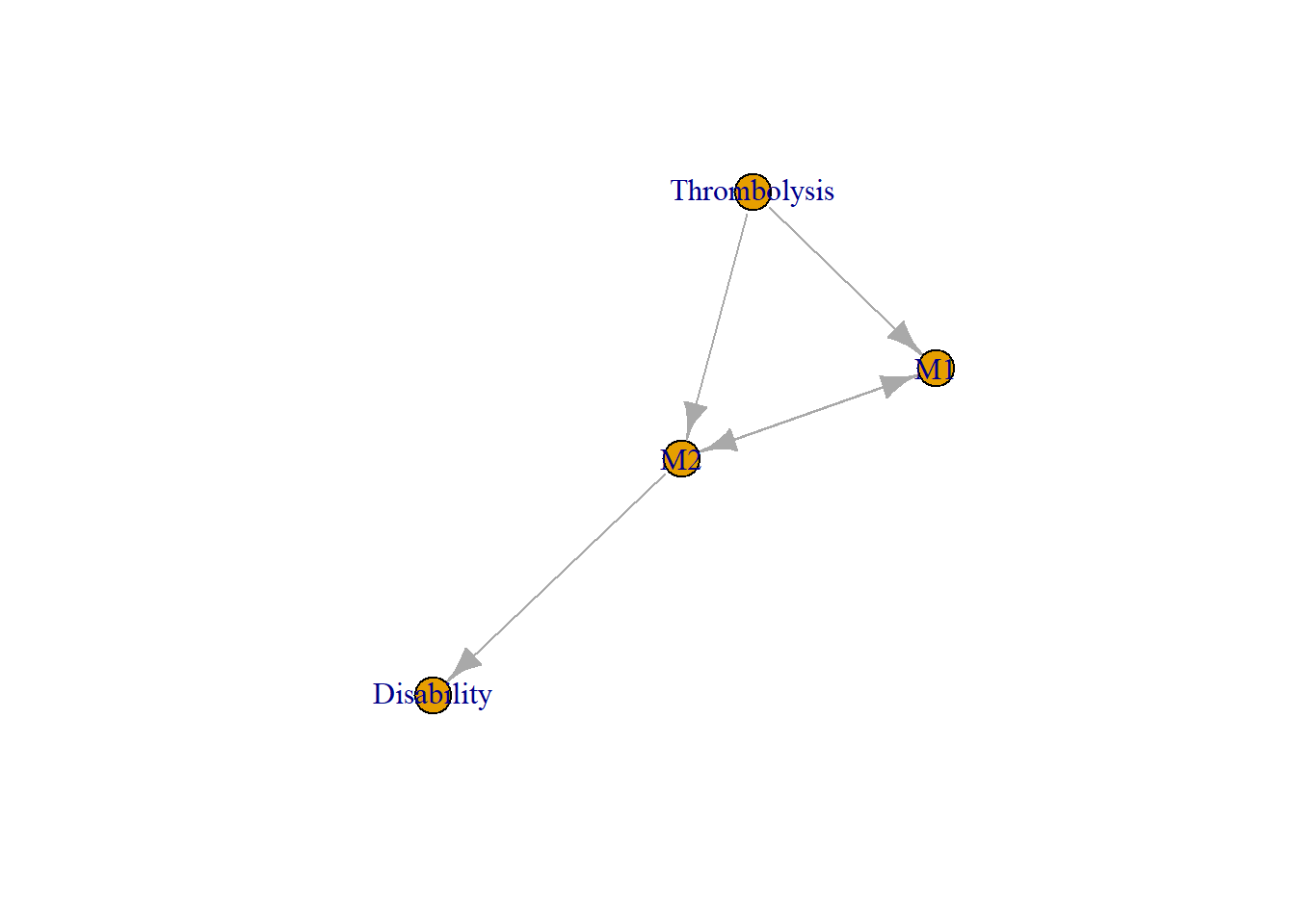
This is a simple example to illustrate different types of matrices from a graph. This graph shows the relationship between ASPECTS region of the brain, thrombolysis and disability outcome (Beare et al. 2015). First we create a network of 4 nodes.
library(igraph)
Attaching package: 'igraph'
The following objects are masked from 'package:stats':
decompose, spectrum
The following object is masked from 'package:base':
union
aspects<-graph(c("M1","M2","M2","Disability","Thrombolysis","M1","M2","M1","Thrombolysis","M2"))plot(aspects) #aspects is the name of the graph
11.1 Special graphs
11.1.1 Laplacian matrix
The Laplacian matrix is the difference between the degree and adjacency matrix. The degree matrix represents the number of direct connection of a node. The diagonal of Laplacian matrix retains the diagonal values of the degree matrix (since the diagonal of the adjacency matrix consists of zeroes).
11.1.1.1 Fiedler value
The smallest eigenvalue of the Laplacian describes whether the graph is connected or not. The second eigenvalue of the Laplacian matrix is the algebraic connectivity or Fiedler value. High Fiedler value indicates greater number of connected components and consequently, resilience to breakdown in flow of information between members(Jamakovic and Mieghem 2008) .
The summary of directed graph from this network is shown here.
Nodes
In-link
Outlink
M1
M2, Thrombolysis
M2
M2
M1, Thrombolysis
Disability
Disability
M2
0
Thrombolysis
0
M1, M2
The degree matrix is generated here from the above network. The explanation for degree centrality is described below.
Degree
M1
3
M2
4
Thrombolysis
2
Disability
1
The adjacency matrix is generated here from the above network.
M1
M2
Thrombolysis
Disability
M1
0
1
1
0
M2
1
0
1
0
Thrombolysis
1
1
0
0
Disability
0
1
0
0
The Laplacian matrix is now generated from the difference between degree and adjacency matrices.
The Markov matrix is generated from the above network. The Markov matrix has the property that the transitional probabilities among the columns of each row sum to ones.
M1
M2
Thrombolysis
Disability
Row total
M1
0
1
0
0
1
M2
0.5
0
0
0.5
1
Thrombolysis
0.5
0.5
0
0
1
Disability
0
0
0
0
0
11.2 Bimodal (bipartite) graph
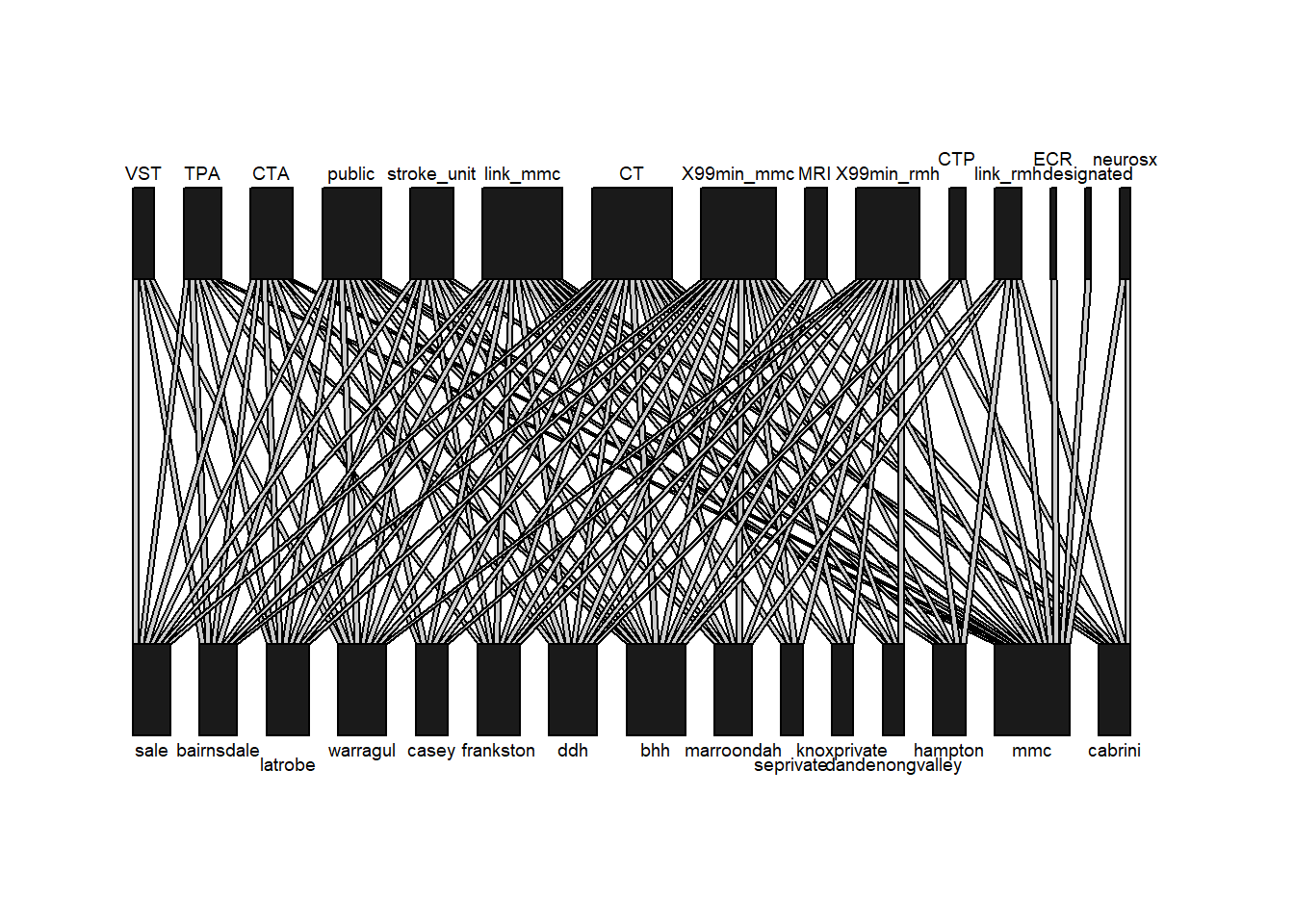
Bimodal graph describes a graph whose vertices can be partitioned into 2 separate sets. It is of interest in social network and in analysis of food ecosystem in nature. A well studied example is the Zachary karate club network. This dataset is included in the igraphdata package. Below we illustrate a bimodal graph of hospitals in South East Melbourne against their characteristics.
library(bipartite)
Loading required package: vegan
Loading required package: permute
Attaching package: 'permute'
The following object is masked from 'package:igraph':
permute
Loading required package: lattice
This is vegan 2.6-4
Attaching package: 'vegan'
The following object is masked from 'package:igraph':
diversity
Loading required package: sna
Loading required package: statnet.common
Attaching package: 'statnet.common'
The following objects are masked from 'package:base':
attr, order
Loading required package: network
'network' 1.18.1 (2023-01-24), part of the Statnet Project
* 'news(package="network")' for changes since last version
* 'citation("network")' for citation information
* 'https://statnet.org' for help, support, and other information
Attaching package: 'network'
The following objects are masked from 'package:igraph':
%c%, %s%, add.edges, add.vertices, delete.edges, delete.vertices,
get.edge.attribute, get.edges, get.vertex.attribute, is.bipartite,
is.directed, list.edge.attributes, list.vertex.attributes,
set.edge.attribute, set.vertex.attribute
sna: Tools for Social Network Analysis
Version 2.7-1 created on 2023-01-24.
copyright (c) 2005, Carter T. Butts, University of California-Irvine
For citation information, type citation("sna").
Type help(package="sna") to get started.
Attaching package: 'sna'
The following objects are masked from 'package:igraph':
betweenness, bonpow, closeness, components, degree, dyad.census,
evcent, hierarchy, is.connected, neighborhood, triad.census
This is bipartite 2.18.
For latest changes see versionlog in ?"bipartite-package". For citation see: citation("bipartite").
Have a nice time plotting and analysing two-mode networks.
Attaching package: 'bipartite'
The following object is masked from 'package:vegan':
nullmodel
The following object is masked from 'package:igraph':
strength
edge<-read.csv("./Data-Use/Hosp_Network_geocoded.csv")#community structure of a network as distinct clusters of interactionsdf<-edge[,c(2:dim(edge)[2])]row.names(df)<-edge[,1] #select columns to remove distance datadf_se<-edge[,c(2:16)]row.names(df_se)<-edge[,1] #select rows to subset south eastern hospitalsdf_se<-df_se[c(1,6,7,11,12,13,14,17,19,20,24,31,33,34,35),]#convert to matrixdf_se_m<-as.matrix(df_se)#bipartite plotplotweb(df_se_m)
This bipartite plot is performed using the bipartiteD3 library.
bipartiteD3::bipartite_D3(df_se_m)
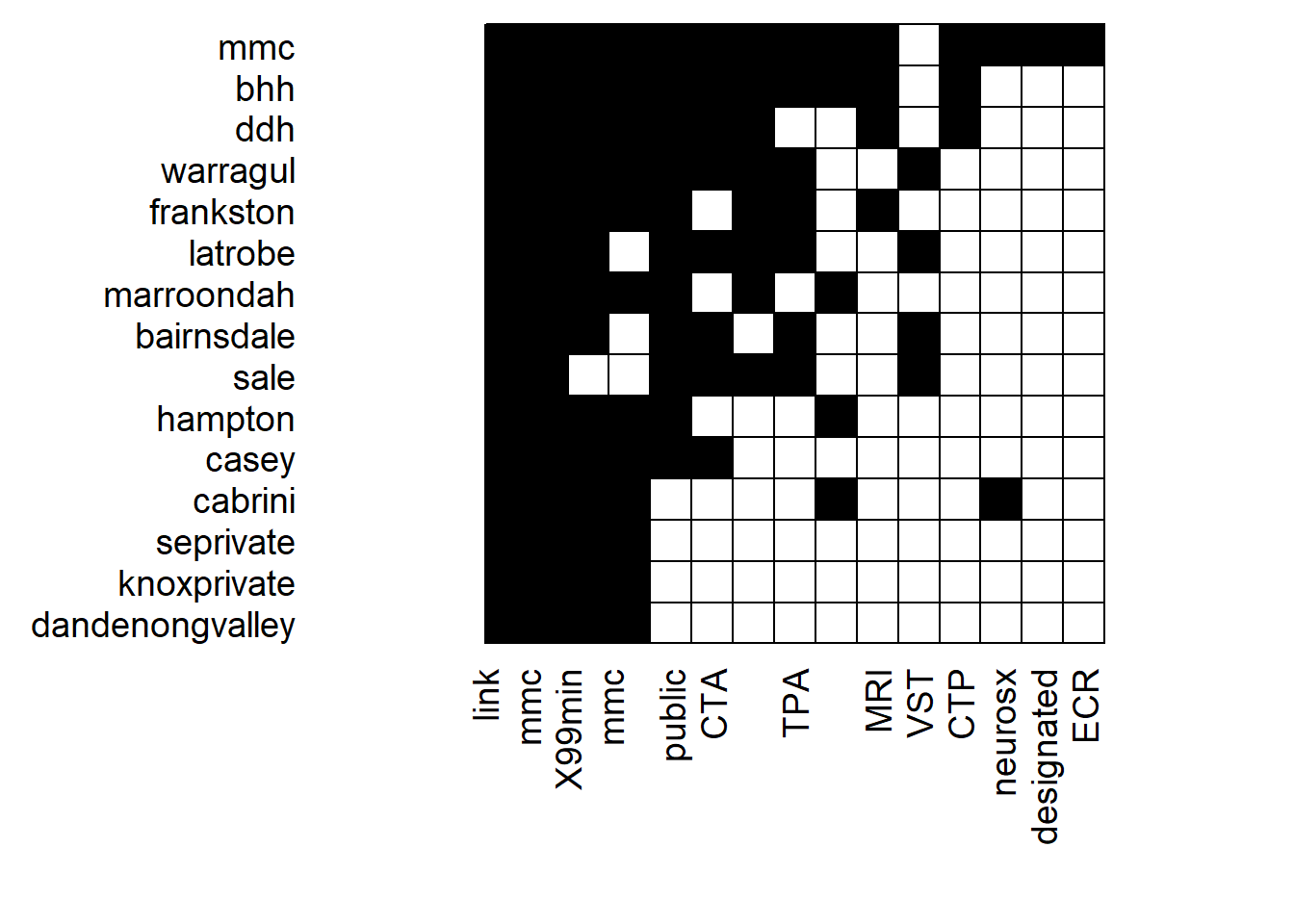
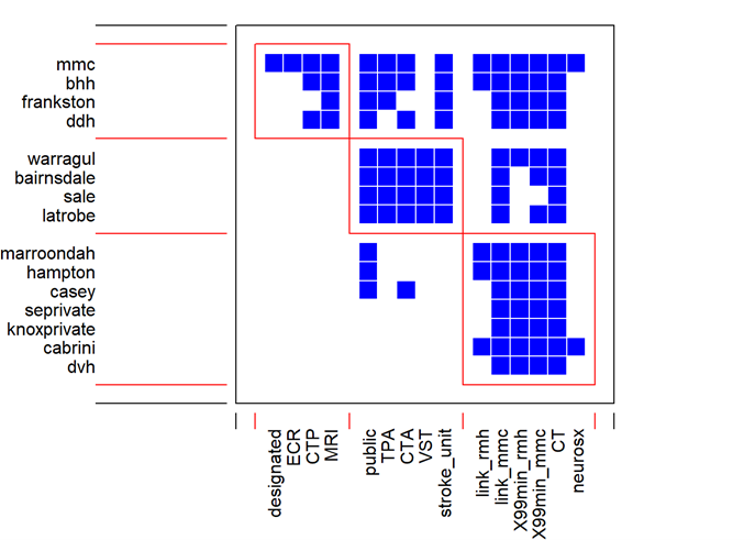
Plot of adjacency matrix of SE hospital network
visweb(df_se_m)
The circular plotPAC examines the potential for competition in parasite network. The width of the line represents the probability.
#plotPAC(df_se_m)
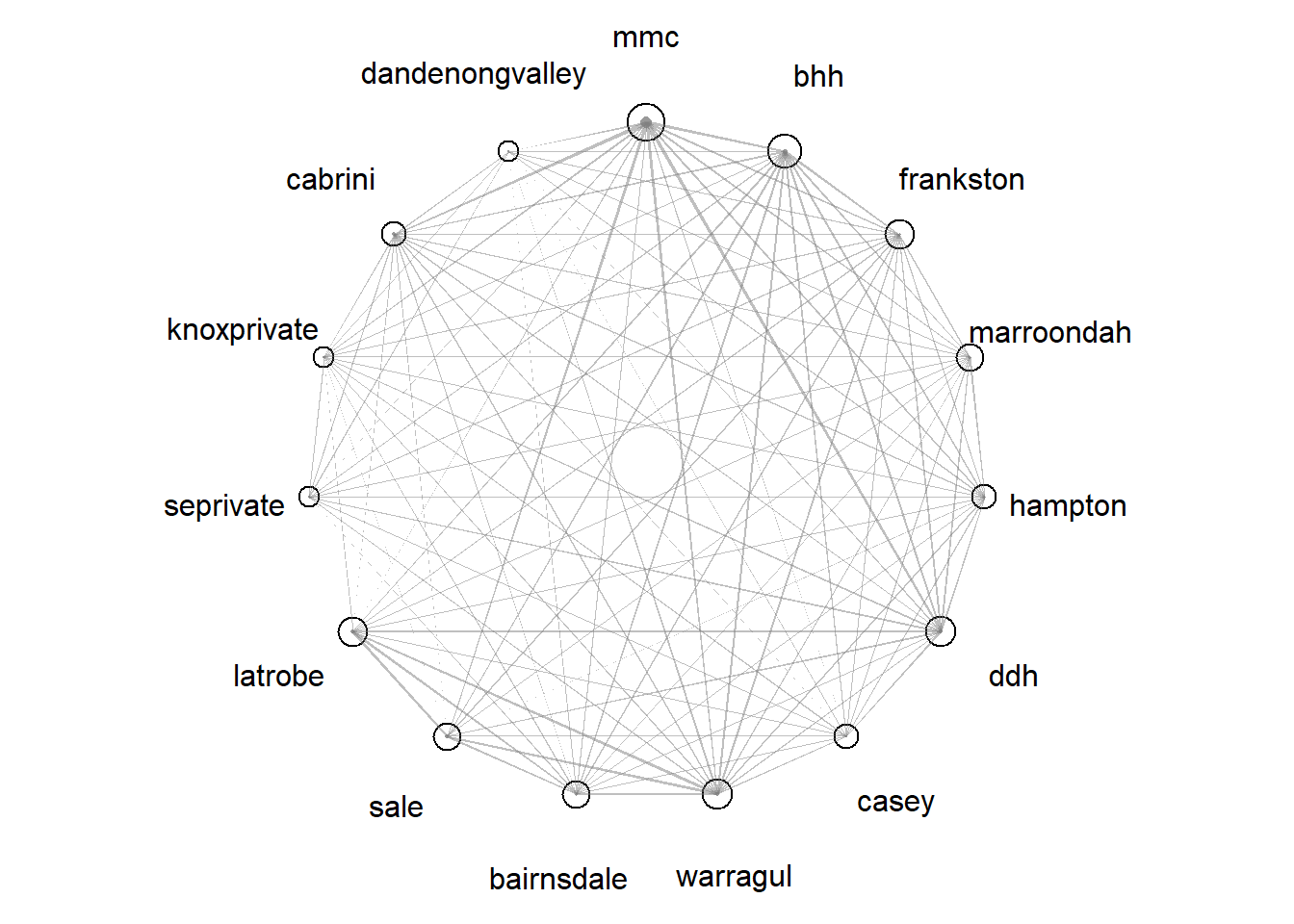
Create community structure of a network as distinct clusters of interactions
Nedge3<-computeModules(df_se)plotModuleWeb(Nedge3) #module web object
SE Hospital Network
library(latentnet)
Loading required package: ergm
'ergm' 4.5.0 (2023-05-27), part of the Statnet Project
* 'news(package="ergm")' for changes since last version
* 'citation("ergm")' for citation information
* 'https://statnet.org' for help, support, and other information
'ergm' 4 is a major update that introduces some backwards-incompatible
changes. Please type 'news(package="ergm")' for a list of major
changes.
Attaching package: 'ergm'
The following object is masked from 'package:statnet.common':
snctrl
'latentnet' 2.10.6 (2022-05-11), part of the Statnet Project
* 'news(package="latentnet")' for changes since last version
* 'citation("latentnet")' for citation information
* 'https://statnet.org' for help, support, and other information
NOTE: BIC calculation prior to latentnet 2.7.0 had a bug in the calculation of the effective number of parameters. See help(summary.ergmm) for details.
NOTE: Prior to version 2.8.0, handling of fixed effects for directed networks had a bug. See help("ergmm-terms") for details.
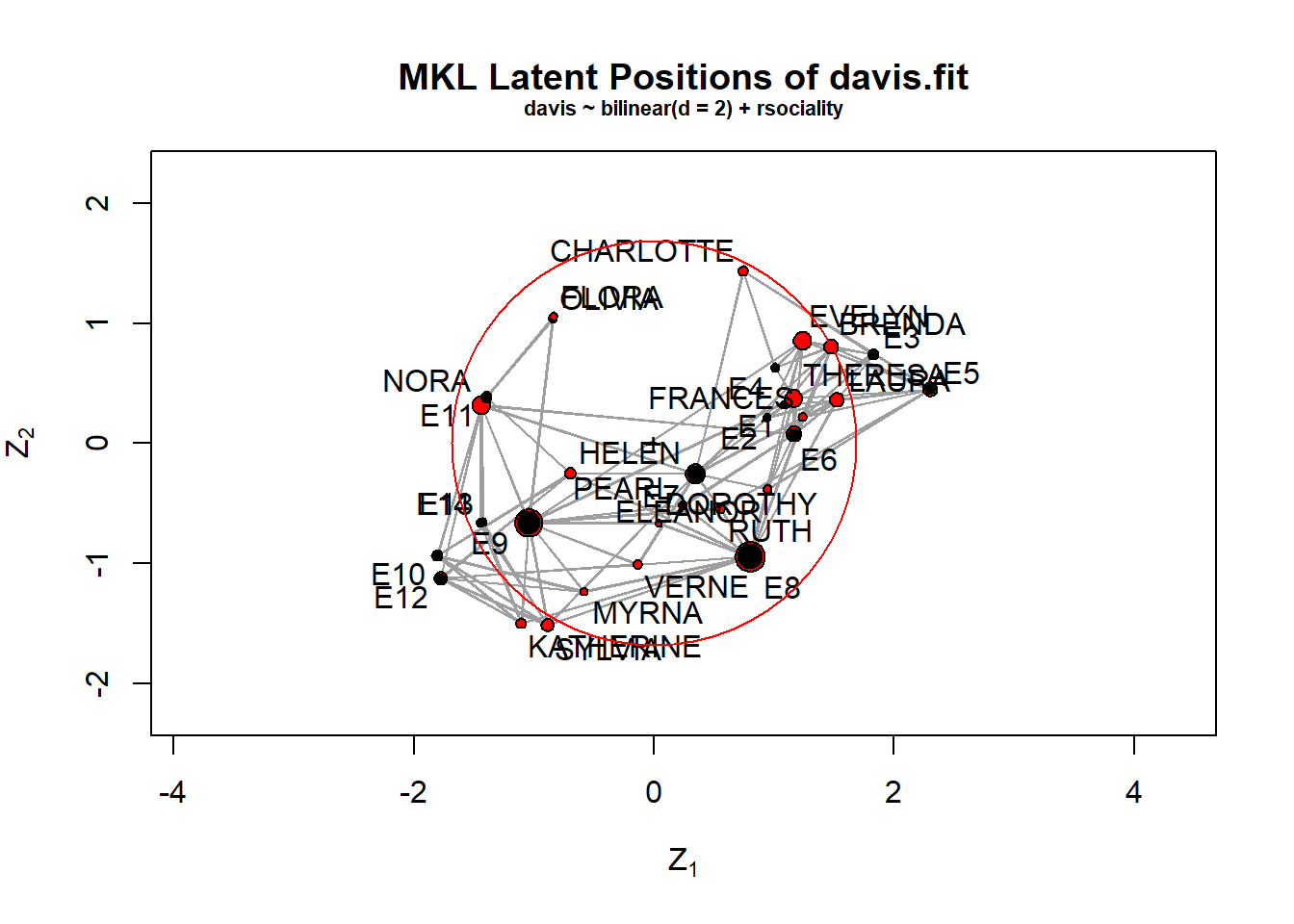
#davis of social networkdata(davis)davis.fit<-ergmm(davis~bilinear(d=2)+rsociality)plot(davis.fit,pie=TRUE,rand.eff="sociality",labels=TRUE)
#davis[,1:10]
11.3 Centrality Measures
In this book, centrality measures are classified as local and central measures.
#the network data is provided above on ASPECTS regions#degree is available in igraph, snad<-igraph::degree(aspects)#closeness is available in igraph, snacl<-igraph::closeness(aspects)#betweennessb<-igraph::betweenness(aspects)#page rankp<-page.rank(aspects)#put data togetherdf<-data.frame("degree"=round(d,2),"closeness"=round(cl,2),"betweenness"=round(b,2),"PageRank"=round(p$vector,2))#formulate tableknitr::kable(df)
degree
closeness
betweenness
PageRank
M1
3
0.33
0
0.29
M2
4
0.50
2
0.37
Disability
1
NaN
0
0.25
Thrombolysis
2
0.25
0
0.09
11.3.1 Local centrality measures
Centrality measures assign a measure of “importance” to nodes and can therefore indicate whether some nodes are more critical than others in a given network. When network nodes represent variables, centrality measures may indicate relevance of variables to a model.
11.3.1.1 Degree centrality
The simplest centrality measure, degree centrality, is the count of links for each node and is a purely local measure of importance. Node strength, used in weighted networks, is the sum of weights of edges entering or leaving (or both) the node.
11.3.1.2 Betweeness centrality
Other measures, such as betweenness centrality, describe more global structure - the degree of participation of a node as conduit of information between other nodes in a network.
11.3.2 Global centrality measures
11.3.2.1 Eigenvector centrality
Eigenvector centrality measure a node’s centrality in terms of node parameters and centrality of neighboring nodes. It works best with undirected graphs. Other forms of eigenvector centrality include alpha centrality and Katz centrality.
11.3.2.2 PageRank
PageRank is one member of a family of graph eigenvector centrality measures. All of these measures incorporate the idea that the score of a node depends, at least in part, on the scores of neighbors connecting to the node. Thus a page may have a high PageRank score if many pages link to it, or if a few important or authoritative pages link to it. PageRank uses a different scaling for connections (by the number of links leaving the node) and importance is based on incoming connections rather than outgoing connections(Brin and Page 1998). Thus a small number of links from influential pages can greatly enhance the importance of the destination page.
PageRank has several differences with respect to other eigenvector centrality methods, expanded below, which make it better suited for digraphs. PageRank was originally described in terms of a web user/surfer randomly clicking links, and the PageRank of a web page corresponds to the probability of the random surfer arriving at the page of interest. The model of the random surfer used in the PageRank computation includes a damping factor, which represents the chance of the random surfer becoming bored and selecting a completely different page at random (teleporting to a random page). Similarly, if a page is a sink (i.e. has no outgoing links), then the random web surfer may click on to a random page.
A number of different approaches are available for computing the PageRank for nodes in a network. The conceptually simplest is to assign an equal initial score to each node, and then iteratively update PageRank scores. This is easy to perform algebraically for a small number of nodes but can take a long time with larger data. In practice, it is performed using eigenvector methode. PageRank analysis can be performed using igraph package. (Beare et al. 2015)
11.4 Community membership
Community membership of a network can be defined using walktrap community (random walk tend to stay in the same community), edge betweenness community (dense connections within the same community).
There are many packages for visualising graph such as igraph, sna, ggraph, Rgraphviz, visnetwork, networkD3.
11.5.1 Visnetwork
library(igraph)library(RColorBrewer)library(visNetwork)#open csv fileedge<-read.csv("./Data-Use/TPA_edge.csv") #3 columns:V1 V2 time node<-read.csv("./Data-Use/TPA_node.csv")#convert data to graphdf<-graph_from_data_frame(d=edge[,c(1,2)],vertices = node,directed=F)V(df)$type<-V(df)$name %in% edge[,1]#assign colorvertex.label<-V(df)$membership# Generate colors based on type:colrs <-c("gray50", "gold")V(df)$color <- colrs[V(df)$membership]#assign shapeshape <-c("circle", "square")V(df)$shape<-shape[V(df)$membership] #extract data for visNetworkdata<-toVisNetworkData(df)visNetwork(nodes=data$nodes,edges=data$edges, main="TPA ECR Network")%>%visNodes(color =list(hover ="red")) %>%visInteraction(hover =TRUE)
11.5.2 NetworkD3
NetworkD3 uses a lot of RAM and hence is turned off here.
library(networkD3)# Convert to object suitable for networkD3athero_d3 <-igraph_to_networkD3(g.1a, group = members)## Create force directed network plotforceNetwork(Links = athero_d3$links, Nodes = athero_d3$nodes,Source ='source', Target ='target', NodeID ='name', Group ='group',opacity =0.8,zoom =TRUE)
11.5.3 Large graph
There are very few softwares capable of handling very large graph with the exception of Sigmajs, Gephi , Cytoscape and Neo4J.
11.5.3.1 Gephi
Gephi takes graphml file from igraph. In Gephi, the node names need to be copy from Name column to Label column in Gephi data laboratory. The graph display is set to Fruchterman Reingold layout and run until the layout is stable. Next, the graph statistics are calculated using the tab ‘statistics’. The ‘modularity class’ output is imported into ‘Filter’ under ‘Attributes: Partition’. Following this, the node size is set according to degree centrality and the node color is set according to modularity class. The interactive graph was generated using Sigma Exporter plugins in Gephi. https://gntem2.github.io/Mining-Literature-Atherosclerosis/.
Before visualisation, a manual editing step for the config.json file is required. The config.json is edited as follow: sigma: drawing Properties: label. The threshold is changed from 10 to 5; sigma:drawing Properties: default Label Size is changed from 14 to 7. sigma: graph Properties: max Edge Size change from 0.5 to 4; sigma: graph Properties: min Edge Size is changed from 0.2 to 0.5; sigma: graph Properties: max Node Size is changed from 7 to 14.
11.5.3.2 Sigmajs
The sigmajs library is a wrapper for sigma.js JavaScript library. It plots graph using WebGL and is faster than with Canvas or SVG (networkD3). It is used here to plot the genes interaction in atherosclerosis. It can take igraph object or gexf (graph exchange xml format) files as input. The library Sgraph is also bassed on sigma.js.
library(sigmajs)
Warning: package 'sigmajs' was built under R version 4.3.3
athero_gexf<-"../../DataMining/Atherosclerosis/Inflammation/athero_network_graph.gexf"sigmajs() %>%sg_from_gexf(athero_gexf) %>%#specify layout from igraphsg_settings(igraph::layout.fruchterman.reingold) %>%#highlight neighbor when clicksg_neighbors() %>%#node by sizesg_relative_size()
Social media platform such as twitter, youtube, facebook and instagram are rich source of information for graph theory analysis as well as textmining. The following section only covers twitter and youtube as both are accessible to the public. There’s restricted access for facebook and instagram.
11.6.1 Twitter (X)
Analysis of Twitter requires creating an account on Twitter. This step will generate a series of keys listed below. These keys should be stored in a secret location. There are several different ways to access Twitter data. It should be noted that the data covers a range of 9 days and a maximum of 18000 tweets can be downloaded each day. The location of the tweeter can also be accessed if you have created an account with Google Maps API.
library(rtweet)create_token(app="",consumer_key="",consumer_secret ="",access_token ="",access_secret ="")# searching for tweets on WHOCW <-search_tweets("WHO", n =18000, include_rts =TRUE)# searching for tweets confined y locationsearchTerm_t= (geocode= ("-37.81363,144.9631,5km"))myTwitterData <-Authenticate("twitter", apiKey=myapikey, apiSecret=myapisecret, accessToken=myaccesstoken, accessTokenSecret=myaccesstokensecret) %>%Collect(searchTerm=searchTerm_t, numTweets=100, writeToFile=FALSE,verbose=TRUE)#alternately confined search for tweets on MS from AustraliaMStw <-search_tweets("multiple sclerosis", geocode =lookup_coords("AUS"),n =18000, include_rts =FALSE)rt <-lat_lng(MStw)#extract lat and lon from tweets## plot lat and lng points onto mapwith(rt, points(lng, lat, pch =20, cex = .75, col =rgb(0, .3, .7, .75)))leaflet::leaflet(data=rt) %>%addTiles () %>%addCircles(lat=~lat,lng=~lng)## plot time series of tweetsts_plot(MStw, "weeks") + ggplot2::theme_minimal() + ggplot2::theme(plot.title = ggplot2::element_text(face ="bold")) ggplot2::labs(x =NULL, y =NULL,title ="Frequency of #MS Twitter statuses from past 9 days",subtitle ="Twitter status (tweet) counts aggregated using three-hour intervals",caption ="\nSource: Data collected from Twitter's REST API via rtweet" )
11.6.2 Youtube
To perform analysis of comments on Youtube, a Google Developer’s account should be created. The api key should be saved in a secret location. The analysis can be done by identifying the video of interest.
Knowledge graph or graph database stores data as nodes, relationship and properties. In a way the Google search engine can be seen as graph database. The network mining literature on atherosclerosis above is an example of knowledge graph. It displays information on gene and relationship after clicking. The library crosstalk can be used to provide information on the nodes.
Beare, R., J. Chen, T. G. Phan, R. K. Lees, M. Ali, A. Alexandrov, P. M. Bath, et al. 2015. “Googling Stroke ASPECTS to Determine Disability: Exploratory Analysis from VISTA-Acute Collaboration.”PLoS ONE 10 (5): e0125687.
Brin, Sergey, and Lawrence Page. 1998. “The Anatomy of a Large-Scale Hypertextual Web Search Engine.”Computer Networks and ISDN Systems 30 (1-7): 107–17. https://doi.org/10.1016/S0169-7552(98)00110-X.
Fornito, Alex. 2016. “Graph Theoretic Analysis of Human Brain Networks.” In Neuromethods, edited by Massimo Filippi, 2nd ed., 119:283–314. Neuromethods 119. United States of America: Humana Press. https://doi.org/10.1007/978-1-4939-5611-1_10.
Jamakovic, A., and Piet Van Mieghem. 2008. “On the Robustness of Complex Networks by Using the Algebraic Connectivity.” In Networking, edited by Amitabha Das, Hung Keng Pung, Francis Bu-Sung Lee, and Lawrence Wai-Choong Wong, 4982:183–94. Lecture Notes in Computer Science. Springer. http://dblp.uni-trier.de/db/conf/networking/networking2008.html#JamakovicM08.
11.6 Social Media and Network Analysis
Social media platform such as twitter, youtube, facebook and instagram are rich source of information for graph theory analysis as well as textmining. The following section only covers twitter and youtube as both are accessible to the public. There’s restricted access for facebook and instagram.
11.6.1 Twitter (X)
Analysis of Twitter requires creating an account on Twitter. This step will generate a series of keys listed below. These keys should be stored in a secret location. There are several different ways to access Twitter data. It should be noted that the data covers a range of 9 days and a maximum of 18000 tweets can be downloaded each day. The location of the tweeter can also be accessed if you have created an account with Google Maps API.
11.6.2 Youtube
To perform analysis of comments on Youtube, a Google Developer’s account should be created. The api key should be saved in a secret location. The analysis can be done by identifying the video of interest.