library(PRISMAstatement)
#example from Spot sign paper. Stroke 2019
prisma(found = 193,
       found_other = 27,
       no_dupes = 141,
       screened = 141,
       screen_exclusions = 3,
       full_text = 138,
       full_text_exclusions = 112,
       qualitative = 26,
       quantitative = 26,
width = 800, height = 800)7 Metaanalysis
During journal club, junior doctors are often taught about the importance of metaanalysis. It is worth knowing how to perform a metaanalysis in order to critique the study. This is an important issue as the junior doctor is supervised by someone who a content expert but not necessarily a method expert. Metaanalysis can be performed for clinical trials, cohort studies or diagnostic studies. As an example, it is not well known outside of statistics journal that the bivariate analysis is the preferred method to evaluate diagnostic studies (Reitsma et al. 2005). By contrast, the majority of metaanalysis of diagnostic studies uses the univariate method of Moses and Littenberg (Moses, Shapiro, and Littenberg 1993). This issue will be expanded below.
7.0.1 Quality of study
All studies require evaluation of the quality of the individual studies. This can be done with the QUADAS2 tool, available at https://annals.org/aim/fullarticle/474994/quadas-2-revised-tool-quality-assessment-diagnostic-accuracy-studies.
7.0.2 PRISMA
The PRISMA statement is useful for understanding the search strategy and the papers removed and retained in the metaanalysis. An example of generating the statement is provided below in R. The example given here is from a paper on the use of spot sign to predict enlargment of intracerebral hemorrhage (Phan et al. 2019).
This example of flow diagram is generated using DiagrammeR.
#https://rich-iannone.github.io/DiagrammeR/graphviz_and_mermaid.html#attributes
library(DiagrammeR)
grViz("
digraph boxes_and_circles {

  # a 'graph' statement
  graph [overlap = true, fontsize = 10]

  # several 'node' statements
  node [shape = box,
        fontname = Helvetica]
  Stroke

  node [shape = oval,
        fixedsize = false,
        color=red,
        width = 0.9]
  Hypertension; 'No Hypertension'

  node [shape= circle,
  fontcolor=red,
        color=blue,
        fixedsize=false]

  Hypokalemia; 'No Hypokalemia'

  # several 'edge' statements
  edge [arrowhead=diamond]

  Stroke->{Hypertension, 'No Hypertension'}
  Hypertension->{Hypokalemia, 'No Hypokalemia'}

}

")
An alternative plot to the diagram above.
## alternative

grViz("digraph flowchart {
      # node definitions with substituted label text
      node [fontname = Helvetica, shape = rectangle]
      tab1 [label = '@@1']
      tab2 [label = '@@2']
      tab3 [label = '@@3']
      tab4 [label = '@@4']
      tab5 [label = '@@5']


# edge definitions with the node IDs
      tab1 -> tab3
      tab1-> tab2
      #tab2->tab3
      tab2 -> tab4
      tab2-> tab5;
      }

      [1]: 'Stroke n=19'
      [2]: 'Hypertension n=10'
      [3]: 'No Hypertension n=9'
      [4]: 'Hypokalemia n=?'
      [5]: 'No Hypokalemia n=?'
      ")
7.0.3 Conversion of median to mean
One issue with performing metaanalysis is that one paper may report mean and another report median age. The formula for the mean is given by \(\frac{a+2m+b}{4}\) where m is the median, a is the upper and b is the lower range (Wan 2014). The variance is given by \(S^2=\frac{1}{12}(\frac{(a+2m+b)^2}{4}+{(b-a)^2})\). This formula requires examination of the data such as the figure to obtain the upper and lower range. These changes are incorporated into meta libray using meatamean function (Balduzzi, Rücker, and Schwarzer 2019). More recently, investigators suggest to also consider the skewness of the data from the 5 number summary data (Shi et al. 2023). The argument method.mean in function metamean is used to specify the method for estimating the mean. In this case we chose the Luo method for illustration Luo (Luo et al. 2018). See the help page by typing question mark before metamean for more options.
library(meta) Warning: package 'meta' was built under R version 4.3.2Loading required package: metadatLoading 'meta' package (version 7.0-0).
Type 'help(meta)' for a brief overview.
Readers of 'Meta-Analysis with R (Use R!)' should install
older version of 'meta' package: https://tinyurl.com/dt4y5drs#NIHSS data from ANGEL large core trial in NEJM 2023
metamean(q1=4,q3=20,median=16,n=230, method.mean = "Luo") Number of observations: o = 230
mean 95%-CI
13.1932 [11.6506; 14.7358]
Details:
- Untransformed (raw) meansHere the same data is used for the McGrath method (McGrath et al. 2020).
metamean(q1=4,q3=20,median=16,n=230, method.mean = "QE-McGrath") Number of observations: o = 230
mean 95%-CI
13.3333 [11.7907; 14.8759]
Details:
- Untransformed (raw) meansThe conversion from median to mean in metafor is performed using conv.fivenum function (Viechtbauer 2010). There is an update on the metafor page as well as discussion on alternate approach. The default method of this function is to use the methods by Luo (Luo et al. 2018), Wan (Wan 2014) and Shi (Shi et al. 2023)
library(metafor)Loading required package: MatrixLoading required package: numDeriv
Loading the 'metafor' package (version 4.2-0). For an
introduction to the package please type: help(metafor)
# example data frame
EstMean <- data.frame(Paper=c(1:4,NA), min=c(1,2,NA,2,NA), q1=c(NA,NA,4,4,NA),
median=c(5,6,6,6,NA), q3=c(NA,NA,10,10,NA),
max=c(12,14,NA,14,NA),
mean=c(NA,NA,NA,NA,7.0), sd=c(NA,NA,NA,NA,4.2),
n=c(30,30,30,30,30))
EstMean Paper min q1 median q3 max mean sd n
1 1 1 NA 5 NA 12 NA NA 30
2 2 2 NA 6 NA 14 NA NA 30
3 3 NA 4 6 10 NA NA NA 30
4 4 2 4 6 10 14 NA NA 30
5 NA NA NA NA NA NA 7 4.2 30EstMean <- conv.fivenum(min=min, q1=q1, median=median, q3=q3, max=max, n=n, data=EstMean)
EstMean Paper min q1 median q3 max mean sd n
1 1 1 NA 5 NA 12 5.356748 2.695707 30
2 2 2 NA 6 NA 14 6.475664 2.940771 30
3 3 NA 4 6 10 NA 6.713000 4.670521 30
4 4 2 4 6 10 14 6.882074 3.546379 30
5 NA NA NA NA NA NA 7.000000 4.200000 30The estmeansd library uses quantile estimation method with qe.mean.sd function when the data available are the median and quartile ranges (McGrath et al. 2020) (McGrath et al. 2022).The approach here is to use simulation to estimate the parameters.
library(estmeansd) Warning: package 'estmeansd' was built under R version 4.3.2#data from ANGEL large core trial in NEJM 2023
res_qe <- bc.mean.sd(q1.val = 13, med.val = 16,
q3.val = 20, n = 230)
res_qe $est.mean
[1] 16.60765
$est.sd
[1] 5.346383The standard error from the mean can be estimated using get_SE function.
get_SE(res_qe) $est.se
[1] 0.511922
$boot_means
[1] 16.81363 17.70573 17.25322 16.68965 15.43824 17.11564 18.11796 16.92338
[9] 16.92265 16.23179 15.93938 16.71749 16.75640 17.37708 17.03605 16.39582
[17] 16.97119 17.69496 17.30576 15.87520 17.61748 16.22867 16.58155 17.04438
[25] 17.08872 16.45316 17.94052 17.02214 16.57671 16.77555 17.35009 15.87208
[33] 17.10651 16.31824 16.13759 16.53999 17.30748 16.47449 16.89822 16.05361
[41] 17.27363 17.19702 16.80610 15.96279 16.66710 16.37764 16.95387 16.50875
[49] 15.26551 17.02463 16.96807 17.10103 17.35495 16.52199 16.31158 16.35126
[57] 15.98616 16.35788 16.73372 15.46890 16.35319 16.63971 16.51076 17.32493
[65] 17.21663 16.47196 16.41258 15.74792 16.94180 17.81914 16.41687 17.33984
[73] 16.68705 15.79897 15.46947 16.86747 17.85769 17.26483 16.90581 16.82520
[81] 16.22772 17.05941 16.36230 18.25723 17.20121 17.48318 16.71191 17.04701
[89] 17.14877 17.49809 16.66904 16.47748 17.39276 16.90478 16.02512 17.08833
[97] 15.78288 15.98745 16.50399 16.98511 15.86781 16.89882 16.68169 16.66547
[105] 16.60206 16.88353 17.16542 16.72605 17.05718 16.69747 16.74478 17.43517
[113] 16.50753 16.95245 17.21397 15.67226 16.66459 16.53994 16.42315 16.41861
[121] 18.08723 16.59523 17.27586 17.12152 16.75492 17.10798 17.67481 16.91149
[129] 16.17914 17.06621 17.40657 17.21561 17.33594 16.66241 16.25615 17.55019
[137] 16.69983 16.85371 16.60996 16.43038 16.60933 16.20434 16.60770 15.75778
[145] 15.18144 16.19923 17.01716 17.33488 17.11453 17.14791 17.46264 17.83026
[153] 16.58917 17.65053 16.38898 17.12049 15.99498 16.34248 17.06064 17.20428
[161] 16.68224 16.68983 17.21821 16.75455 16.63443 17.60697 16.69765 17.13788
[169] 17.17097 17.33940 18.35737 17.04557 16.48690 16.70502 18.02948 17.00531
[177] 16.39797 17.10141 17.14550 16.01373 16.61533 16.43245 17.02988 17.14876
[185] 16.83365 16.61042 17.11387 17.59733 16.62166 17.05315 16.61816 16.07293
[193] 15.84520 16.71162 15.69940 16.58437 16.18987 16.93207 16.44812 15.85631
[201] 15.49810 16.62578 16.96787 17.35099 16.36768 17.24907 16.95132 15.54237
[209] 17.24798 16.98224 16.94756 16.61497 16.41858 17.10296 16.95468 17.00647
[217] 15.92030 16.74280 15.57529 16.19345 16.69585 17.13755 16.06925 15.70919
[225] 16.35179 17.27058 16.12881 15.99476 17.51314 16.30205 17.69046 16.27237
[233] 16.34596 16.70872 15.76828 17.39713 16.84156 17.17515 16.22970 16.91198
[241] 16.45958 16.36396 17.67427 16.74273 16.02101 16.92285 16.85702 16.84431
[249] 16.66843 16.50790 17.08529 16.84360 16.83592 16.94927 17.27962 16.81046
[257] 17.76496 15.99211 16.65273 16.14989 17.61215 15.73675 16.45889 16.87816
[265] 16.57544 16.97355 17.61647 16.96009 16.91074 16.61190 17.27554 16.21252
[273] 17.38893 16.17475 17.43663 17.17697 16.64691 16.21228 16.79808 17.00444
[281] 16.98334 16.83866 16.32994 16.77004 16.30464 15.64289 16.61921 16.70109
[289] 15.83331 16.99415 16.82635 16.70980 17.30768 16.91957 16.53200 16.98076
[297] 16.80959 15.66606 16.85876 17.05212 16.45794 16.74514 15.64543 16.86062
[305] 16.94205 16.63708 16.44814 16.07887 17.06905 16.00507 17.35612 16.65201
[313] 17.79226 15.62529 16.05805 16.89135 16.54750 16.57772 16.28147 16.02344
[321] 16.53603 16.22986 17.00812 16.78853 17.19983 17.00679 16.62885 16.85799
[329] 16.78650 16.54815 16.91762 17.14785 16.11757 17.52721 17.03673 17.18557
[337] 15.92104 17.07190 16.27448 16.77899 16.01494 17.46099 17.09177 16.24782
[345] 16.65035 15.99515 16.62779 16.46325 17.54684 16.88992 17.08283 16.74426
[353] 16.49304 17.54410 16.45047 17.28483 16.54583 16.87754 16.06437 16.02002
[361] 15.95595 16.57995 16.24122 17.15723 16.78909 16.98413 17.06424 16.77706
[369] 17.33562 16.80102 16.71253 17.49662 16.89484 17.59427 17.12562 15.95079
[377] 17.41755 17.56594 16.54042 17.22069 16.67746 17.14220 16.16774 16.25709
[385] 16.10472 17.39467 16.92708 16.54470 17.52797 16.69332 15.85490 17.16890
[393] 16.81852 15.68845 16.97350 16.66436 16.44133 17.67531 17.11306 15.82517
[401] 17.49350 16.67375 17.38343 16.58596 17.09261 15.65313 17.15474 16.93688
[409] 16.75204 16.58774 16.61994 17.47982 17.22870 16.74318 16.54863 16.84109
[417] 16.83811 17.08684 16.91966 15.98193 17.18413 17.03949 17.15550 16.29706
[425] 17.03456 16.71888 16.72859 16.77195 16.65380 17.06562 16.73286 16.63461
[433] 15.98452 16.86568 17.01868 15.99323 17.05604 16.30280 17.23114 16.90986
[441] 16.41641 16.72895 17.09790 16.24928 17.23502 16.54832 17.28934 16.39340
[449] 17.10240 17.19934 16.32762 16.37589 16.76552 17.31412 15.77307 16.56493
[457] 16.80992 16.52795 16.92869 16.62724 17.18153 16.46647 17.38058 16.79845
[465] 16.37142 17.54235 17.60510 17.39469 16.78431 17.30034 16.85539 17.69922
[473] 17.05348 16.34858 16.42981 17.09941 17.04928 16.95645 16.48778 16.06399
[481] 16.47032 16.51855 17.56933 17.12102 17.73825 16.88866 16.51530 16.64002
[489] 17.28735 16.30843 16.53886 17.58680 16.39208 16.39649 17.12668 17.49574
[497] 15.78733 16.92647 16.60118 16.79645 16.97817 17.42461 16.36224 17.04883
[505] 16.45389 16.50887 17.20279 16.88233 16.93681 16.43726 16.66534 16.95825
[513] 15.78834 17.36306 17.16007 16.89824 16.61537 16.88974 15.93043 16.49377
[521] 16.89677 16.28873 16.04158 16.73035 16.37107 16.76089 17.07279 16.18189
[529] 15.96264 16.74737 16.75586 17.01110 16.80728 16.37744 16.97725 17.08748
[537] 16.48311 16.50263 17.10441 15.97717 17.16944 16.43781 17.17954 16.35494
[545] 16.65786 17.78332 17.00643 16.89675 17.14450 16.97757 17.18080 16.02174
[553] 17.60855 16.35717 16.11633 16.24547 16.19627 17.09202 16.47569 16.91980
[561] 15.94477 16.87288 16.06275 17.25975 15.93478 16.87811 16.22291 16.51310
[569] 16.10228 17.31132 16.43666 17.26297 17.30509 16.74178 17.78746 16.61417
[577] 16.75673 16.86069 17.25876 16.19292 16.01208 16.45491 16.76278 16.67559
[585] 16.57160 17.33251 16.47113 17.02101 16.65191 16.83094 16.68965 16.71971
[593] 16.49964 17.15175 16.64079 17.27504 16.56548 17.11320 16.35525 17.51435
[601] 17.31367 17.40693 16.26688 16.81753 16.99620 17.01423 17.12967 17.18579
[609] 17.03770 17.30052 17.12384 17.73090 16.48327 16.64851 16.74669 17.00479
[617] 16.56992 16.76587 17.26355 16.73507 16.37898 16.66362 17.25961 17.25434
[625] 17.35107 16.37612 15.67531 16.45598 16.65372 17.75589 16.73725 17.19470
[633] 17.23154 16.99428 16.73197 16.97013 16.59185 16.34813 17.47328 17.02556
[641] 16.68052 17.36877 17.66107 16.27058 16.54168 17.28663 16.23500 17.43937
[649] 16.90496 16.97232 16.96093 17.22229 16.95983 17.21452 16.25364 16.95289
[657] 17.37829 17.48408 15.73014 17.47471 16.43506 17.41563 16.29287 16.24110
[665] 16.65883 16.82966 15.91061 16.33051 16.66107 15.81750 16.01074 17.26374
[673] 17.08782 16.37972 16.69085 17.01332 17.15964 16.70982 17.78528 17.43005
[681] 16.38329 16.16270 16.09983 17.22694 16.54410 17.05089 18.00719 15.93033
[689] 17.89228 16.64645 17.46426 16.91659 17.47375 16.23768 15.95120 17.31426
[697] 16.42970 16.47638 16.71497 16.53997 16.29457 16.24483 16.19349 16.52672
[705] 17.24746 16.56309 16.23782 15.96367 16.66385 16.58526 17.51738 16.72092
[713] 16.81471 16.69272 16.36605 15.64328 16.66814 17.16261 17.05237 17.38842
[721] 16.55044 16.97570 16.81594 16.12099 17.64001 16.50747 16.42596 16.91308
[729] 16.68169 16.23597 16.39301 16.24087 17.48447 16.63566 16.81779 17.05690
[737] 15.99294 16.69725 16.57859 16.82712 16.32352 17.22129 16.57544 17.23693
[745] 16.69382 15.85041 16.43885 15.83502 15.87749 16.21703 16.14586 17.53110
[753] 17.23793 16.76503 16.31904 15.43125 16.48912 16.78148 16.51630 17.07357
[761] 16.59499 16.44409 17.73457 17.28955 16.57841 16.97146 15.88039 15.72187
[769] 17.51777 16.21583 16.72176 17.77118 17.71779 17.06883 16.49900 16.22250
[777] 16.13066 16.93482 16.44700 16.78085 16.78296 16.92098 16.71033 17.02038
[785] 15.71967 16.38611 16.46811 16.37434 16.48573 17.08402 17.13443 16.98294
[793] 16.76644 16.85112 16.52553 16.67465 17.23942 15.66688 17.69698 16.89367
[801] 17.13950 17.82964 17.69766 16.13876 16.10389 16.71310 15.87336 17.18304
[809] 16.65223 17.29057 16.96987 17.36303 16.93389 16.80236 16.67906 16.44260
[817] 16.76699 16.19217 17.08444 16.76430 16.26633 16.39913 17.65198 16.97874
[825] 16.84277 17.85136 16.67322 16.01476 17.32004 16.15548 16.60245 16.24125
[833] 15.72331 17.13025 17.51885 16.64169 16.40086 16.90820 17.28666 16.89979
[841] 17.32905 16.39008 16.98701 17.86120 16.44339 16.79400 16.63208 16.56070
[849] 16.75721 17.32020 17.21522 17.36297 16.75481 16.91101 15.90252 16.99672
[857] 16.78798 16.66961 16.70352 17.14832 17.68025 16.59975 16.54618 16.92641
[865] 16.82069 16.16281 16.45609 17.10836 16.90713 17.04006 16.09334 16.56354
[873] 17.17903 16.97747 16.38911 16.22876 17.17173 16.63205 16.55289 16.33554
[881] 16.25505 17.26376 16.55373 15.66381 16.75110 17.82834 17.81719 16.89680
[889] 16.74933 15.90259 16.90617 16.77111 16.98710 17.12510 16.59841 16.53155
[897] 17.31997 16.79606 16.20567 16.45007 16.85927 16.83931 16.30468 15.54803
[905] 17.27780 16.10220 16.36623 17.11615 16.59151 16.56268 16.70685 17.15752
[913] 16.58651 16.88587 17.38102 16.49643 17.31281 16.86435 17.48918 16.70927
[921] 16.59618 16.63401 17.54210 17.36700 16.65976 16.53648 16.90595 16.64727
[929] 17.15273 16.56091 16.32219 16.72035 16.35274 16.89710 16.73029 15.85560
[937] 17.14590 16.60621 16.36167 17.03959 16.66991 17.24809 16.36166 17.01489
[945] 17.37262 16.73975 16.61845 16.41688 16.29759 17.10271 16.84209 16.42369
[953] 16.75713 16.92989 17.28137 17.79838 16.72262 16.50048 16.55710 16.36806
[961] 16.92524 16.34075 16.27410 17.46757 16.92186 16.27089 15.86532 16.93609
[969] 17.17273 16.93433 17.54233 16.08247 17.38850 16.22411 15.77167 15.98179
[977] 16.80016 17.22454 16.50427 17.23994 18.29112 16.00300 16.91659 16.56146
[985] 16.08334 15.89792 17.17740 16.28704 15.41303 16.79503 16.85902 15.78552
[993] 16.54712 17.08107 16.45742 17.10309 17.05863 15.84528 16.91197 17.45227
$boot_sds
[1] 5.323367 6.188049 5.829824 5.283758 4.445092 5.282802 7.077455 5.473896
[9] 5.407557 5.184466 4.911659 5.364991 5.248512 5.225366 5.416984 5.512195
[17] 6.163062 6.697831 5.667194 5.102778 6.845542 4.864111 5.416105 5.956041
[25] 5.768485 5.186732 6.152174 6.410232 5.985907 5.262913 6.011813 4.661363
[33] 5.396243 5.377659 4.808801 5.408405 4.977856 5.485376 6.227896 5.001365
[41] 6.000504 6.297895 5.227609 5.077416 5.668005 5.047082 5.826484 5.004870
[49] 4.886724 5.939368 5.574197 5.711359 6.545391 5.255155 4.931867 5.584749
[57] 5.269086 5.171474 5.001013 4.807262 4.960217 5.394250 5.308097 5.842775
[65] 6.152999 4.546332 4.633818 4.686823 5.206128 6.756992 5.686539 5.541675
[73] 4.870060 4.820766 4.628484 4.926237 4.924015 5.512847 6.101680 5.182194
[81] 5.317645 5.884310 4.548573 6.278788 5.579946 5.102893 4.740109 5.481771
[89] 5.344570 5.277119 5.252014 5.400783 5.856259 5.479254 4.950194 6.298666
[97] 5.170917 5.320271 4.905866 6.038757 4.959091 4.900016 5.216701 5.063830
[105] 4.932071 5.047289 6.459660 5.052633 5.331702 5.051951 6.341675 6.594618
[113] 4.947162 5.960100 5.997420 4.350006 5.368190 5.404501 4.907735 4.816424
[121] 6.846713 5.109606 5.448617 5.246659 5.220453 5.367834 4.891664 5.830699
[129] 5.139512 4.911249 5.120978 5.501816 5.091461 5.124579 4.712670 5.664835
[137] 5.158644 5.636747 5.903465 5.633452 5.061357 5.285733 5.843434 5.046254
[145] 5.370901 4.782595 5.438126 5.376869 5.268480 5.964862 5.946379 6.773504
[153] 4.697600 6.474817 4.926364 5.720071 4.855188 5.482948 6.154577 5.590988
[161] 5.197344 5.444280 6.548397 5.478054 4.443605 5.850116 5.125962 6.301562
[169] 5.859171 5.245949 6.732769 5.094638 4.858793 5.308582 6.665378 6.153753
[177] 5.311860 5.506991 5.616681 4.812815 5.519026 4.645962 5.672307 5.249681
[185] 5.577254 5.350236 5.802556 6.471347 5.105032 5.004560 5.211054 4.552604
[193] 5.176681 4.516261 5.222474 5.085689 4.784406 5.437635 5.358878 4.691885
[201] 4.870214 5.040140 5.302138 5.318178 5.444848 5.879195 6.263393 4.966542
[209] 5.824275 5.951854 6.001998 5.617949 4.804295 5.980560 5.140736 5.871422
[217] 5.364605 5.675486 5.029280 4.620212 5.165263 5.504987 5.194528 5.086301
[225] 4.930638 6.622517 4.968458 4.753982 6.051637 4.733573 5.981452 4.804698
[233] 4.886838 5.954339 4.943127 5.682809 5.843325 6.366458 4.850147 5.342727
[241] 5.190235 5.306626 6.038010 5.545958 5.221102 5.206749 5.942433 5.004228
[249] 6.420307 5.341143 5.270173 5.026164 5.466866 5.767927 6.230660 5.822404
[257] 6.438979 5.607596 5.086969 5.359944 7.106908 4.558682 5.876763 5.157863
[265] 4.965119 5.176577 5.984971 5.808632 5.575939 5.295249 5.403636 5.351762
[273] 5.548143 4.347757 5.889505 5.884569 5.027002 4.440748 5.912612 6.017948
[281] 5.016638 5.557467 5.226442 5.701534 5.370018 5.390881 4.333008 5.323570
[289] 5.440303 6.264274 5.688107 5.238662 4.719242 6.012436 4.868774 5.411649
[297] 5.084997 5.365931 5.254247 6.032297 4.855674 4.944614 4.825227 5.807302
[305] 5.177797 4.870605 4.749347 5.474619 6.297992 5.262023 5.318316 5.441403
[313] 6.491753 4.112387 5.101388 5.397310 5.380438 4.668946 4.793648 4.659688
[321] 4.699530 4.948507 5.312955 5.526283 5.728054 6.658549 5.752019 6.025745
[329] 5.340052 5.146366 5.614515 5.576403 4.654336 5.975398 5.222328 5.692318
[337] 3.671859 5.848328 5.443980 5.571770 4.711341 5.824472 5.953412 4.824465
[345] 5.054990 5.151502 4.415276 5.739008 6.652707 5.905736 5.253249 5.854966
[353] 5.456577 6.597252 5.066676 5.353384 5.627671 5.750642 4.520376 4.919176
[361] 4.380013 5.930292 4.929376 5.927135 5.992668 5.865287 5.239742 5.638240
[369] 5.630076 5.040397 5.957226 6.337194 4.582010 5.810570 5.746842 4.769660
[377] 6.896101 6.148152 6.120831 5.620568 6.045299 5.423197 5.255632 4.955501
[385] 4.834296 5.710168 4.057176 5.067770 5.659783 4.967594 5.551340 5.743152
[393] 5.038279 5.328960 5.863009 5.042017 5.498558 5.539242 6.037138 4.631512
[401] 6.082863 5.379845 6.297969 4.946708 5.892848 4.275836 5.984897 6.241082
[409] 5.615182 5.394902 5.123052 5.522997 5.884988 5.515392 5.034922 6.061200
[417] 4.919157 5.162753 6.240256 4.182514 5.437950 5.480062 6.144158 5.887565
[425] 4.741429 5.186499 5.201342 5.356954 5.158240 5.133530 4.017774 5.934152
[433] 5.037753 6.068374 5.527881 4.377188 5.937209 5.041319 6.759797 5.443339
[441] 5.580607 5.408991 5.296448 4.731205 5.809822 4.916460 5.519138 5.635915
[449] 5.689952 5.272039 4.843322 4.808495 5.085973 5.351774 4.638639 5.335906
[457] 5.087387 5.033105 5.807488 6.087083 5.924421 5.083133 5.660980 5.106142
[465] 5.109707 5.847873 5.929322 6.608877 6.239915 5.731330 5.808553 6.051780
[473] 5.041159 4.797416 5.206871 6.727443 6.001875 4.731066 4.766156 5.775015
[481] 5.379651 5.277713 6.098697 5.686521 5.771156 5.032150 5.012877 5.120146
[489] 5.676641 5.103607 5.090446 5.631484 5.036104 5.179831 5.951367 5.468116
[497] 4.647818 6.125980 5.426655 5.393820 5.762161 5.803353 4.760084 5.971601
[505] 5.015802 5.274803 5.090428 4.926898 5.948179 5.285476 5.514665 6.061820
[513] 4.116867 6.086825 5.789307 5.542555 5.099026 5.588184 5.668445 5.064272
[521] 6.507418 4.322272 5.437230 5.024152 5.239046 5.346567 5.516487 4.913103
[529] 4.885650 4.775886 5.261077 6.218143 5.424767 4.490387 4.728488 5.803381
[537] 4.871424 5.115799 5.602586 4.734766 6.137642 5.177178 5.893637 5.425322
[545] 5.509729 6.599464 5.849066 5.893025 5.519609 5.627698 5.736211 4.853406
[553] 5.558310 4.975814 5.001299 4.994162 5.285768 5.115328 5.199442 6.056987
[561] 4.166357 4.953992 3.998926 5.254724 5.039581 4.834401 6.116325 4.539656
[569] 4.805686 5.978977 4.990576 5.910541 5.727773 6.200043 6.396726 5.753578
[577] 5.165451 5.580264 6.621164 5.082948 5.076846 5.062512 5.019345 4.855833
[585] 5.173368 6.441898 5.755693 5.303293 5.439128 6.225915 6.255661 5.972276
[593] 5.404084 5.674569 5.385654 5.407062 4.866443 5.564455 4.832618 6.178218
[601] 5.243314 6.388612 4.814762 5.967683 5.466384 4.915170 6.180645 5.872415
[609] 5.831054 6.145136 5.772405 6.667228 5.506139 5.379110 4.717256 6.063017
[617] 5.686468 5.732996 5.794095 5.477455 4.409884 5.453401 6.028773 5.462014
[625] 5.846211 4.335593 5.017042 4.861328 5.473062 6.729320 5.386894 5.342770
[633] 5.422600 5.761749 5.846457 5.061213 5.539820 5.113684 5.717678 5.514253
[641] 5.440647 6.404056 6.257627 5.553710 5.514372 6.511028 5.061438 6.165014
[649] 5.070590 5.047284 5.030606 4.683583 5.520954 5.772016 5.449320 5.138231
[657] 5.409202 5.262760 4.873857 6.126843 6.005227 5.114987 4.910225 5.286108
[665] 6.126636 5.570519 4.952508 5.241042 4.977953 4.460684 4.964115 5.757605
[673] 6.132008 4.386284 5.446997 6.505078 5.470974 5.195875 5.980432 5.774611
[681] 5.067232 5.249879 5.219937 6.565196 6.099162 4.729982 6.803301 4.445915
[689] 6.317268 5.612088 5.885416 5.021010 5.501904 5.474699 4.641883 5.501650
[697] 5.294283 5.029124 5.785695 5.554118 4.850048 5.124206 5.241084 5.965215
[705] 5.480994 5.435805 4.692504 5.116168 4.960773 4.933634 5.829885 6.001924
[713] 5.267723 4.708574 5.183844 4.267713 5.358690 4.925114 4.784024 5.751247
[721] 5.079363 5.468452 5.450708 4.747455 6.909489 5.141674 5.455227 5.690618
[729] 5.676269 4.918785 5.137197 5.520243 5.522385 5.046100 5.407013 6.291335
[737] 5.425717 5.384007 5.411508 5.094698 5.166057 6.185594 5.493574 5.981302
[745] 4.778106 4.976319 4.977921 4.681386 4.888936 4.201670 5.202099 5.206625
[753] 5.832878 5.767608 5.677991 4.860917 4.936702 5.050055 5.950608 6.096555
[761] 5.982158 5.897432 6.877524 6.227898 4.906355 5.436202 4.729186 4.485784
[769] 6.820576 4.433259 5.832036 5.523445 5.962459 5.413728 4.951561 4.940542
[777] 5.256753 5.757410 4.965982 4.812575 4.868448 6.091936 4.871047 6.051793
[785] 4.514362 4.736419 5.103924 4.957530 4.968336 5.297408 5.085033 5.420658
[793] 4.558831 4.969573 5.953207 5.397718 7.112402 4.459641 5.249264 4.885358
[801] 5.589794 5.573605 6.050769 4.750015 5.119709 4.315271 4.554800 5.417566
[809] 5.083104 5.822150 4.968353 6.152950 5.792442 5.488435 5.710975 6.165191
[817] 5.277695 5.084423 6.151215 5.720073 4.752673 5.316098 6.217598 5.256085
[825] 5.257717 5.958119 4.967623 5.506812 6.276196 5.020024 5.043128 5.049569
[833] 5.231644 5.743037 4.976123 6.053969 5.742857 5.148854 6.329220 5.343864
[841] 5.586979 5.788614 6.211011 5.546672 5.641508 4.782922 5.022193 5.197027
[849] 5.497562 6.443563 5.461792 5.434378 5.146162 6.713887 4.883125 5.362630
[857] 6.191950 5.172578 5.543222 6.610082 5.629794 5.135476 5.238716 5.764892
[865] 5.452481 5.409279 5.530629 5.639668 5.219238 6.050555 4.490161 5.590892
[873] 5.852444 5.375741 5.173974 4.396516 6.056490 5.938530 5.236136 5.742804
[881] 4.798472 5.010959 6.019005 4.623430 5.734139 6.230055 6.433471 5.646349
[889] 5.702253 4.689224 5.134936 5.416108 5.564481 5.697215 5.864516 5.310785
[897] 5.939809 6.027458 4.879879 5.793371 5.726668 4.913424 4.505511 4.675124
[905] 6.520513 4.755512 5.807141 5.899656 5.229531 5.038139 4.699273 6.068936
[913] 5.479134 5.100078 5.651096 5.571576 5.836229 5.042473 6.264833 5.306091
[921] 4.741963 4.737254 5.270891 6.725771 5.209795 6.354659 5.159849 5.226417
[929] 4.745801 5.573936 5.034987 5.052598 5.302433 5.147203 5.309981 4.389330
[937] 5.200957 5.332901 5.095185 5.631112 4.971977 5.985898 5.327254 6.234480
[945] 6.160403 5.385406 4.957520 5.148128 4.779292 5.901769 6.757535 4.479893
[953] 4.551883 4.937486 6.045153 6.312790 5.384144 5.022228 5.314678 5.661734
[961] 6.126895 5.839106 5.127379 5.685349 5.588283 5.094462 4.576997 4.884910
[969] 5.250479 5.368456 5.875731 5.646250 5.620271 4.792648 5.038888 4.378607
[977] 4.805374 5.507174 5.030463 5.440528 6.232720 4.578207 5.622868 5.676263
[985] 4.394518 5.122867 5.868749 5.748056 4.579322 6.003500 5.050304 5.304506
[993] 4.655752 6.099608 5.527444 5.687799 5.741733 4.857653 5.790900 5.490219The estmeansd library uses Box-Cox method for estimating mean and sd when the data available are the median, minimum and maximum values.
library(estmeansd)
res_bc <- bc.mean.sd(min.val = 13, med.val = 16,
                     max.val = 42, n = 230)
res_bc
$est.mean
[1] 16.7176
$est.sd
[1] 3.519021Again, the standard error from the mean can be estimated using get_SE function.
get_SE(res_bc) $est.se
[1] 0.3052039
$boot_means
[1] 16.98197 16.47295 16.92522 16.96211 16.15494 16.91716 16.83265 16.66382
[9] 17.11220 17.29621 16.84693 16.69995 16.87783 16.53914 16.46023 16.75153
[17] 16.94374 16.30851 16.52389 16.28983 16.55618 16.83480 16.79055 16.70403
[25] 16.55713 16.80955 16.42885 16.61581 16.49591 16.47304 16.22143 16.88442
[33] 17.17244 16.76734 16.16497 16.66508 17.36709 16.48286 16.59040 16.67506
[41] 16.67032 16.48246 16.76786 16.89323 16.61967 17.07082 16.65678 17.09284
[49] 16.36550 16.64437 16.74867 16.70292 16.68246 16.74257 16.56080 16.55009
[57] 16.49339 16.81383 16.20580 16.91572 16.80273 16.56303 16.92206 16.62915
[65] 17.02097 16.72551 16.66004 17.09384 16.80036 16.58135 16.35111 16.97333
[73] 16.14641 16.86625 16.58425 17.03519 17.36464 17.32702 16.59844 16.98146
[81] 17.21575 16.67543 16.85970 16.99978 17.29157 16.79706 16.48221 16.61820
[89] 16.55372 16.73765 17.00646 16.92399 16.98630 16.40824 16.99410 16.53783
[97] 16.15655 16.53336 16.43541 16.94859 16.92463 16.88376 16.30601 16.13211
[105] 16.29156 16.56867 16.32783 16.68535 16.58206 16.94852 16.14591 16.51675
[113] 16.65870 16.99033 16.87511 16.78819 16.79958 17.47929 16.86430 16.50682
[121] 16.66867 16.23941 16.73048 16.18795 16.89135 16.82558 17.15043 16.70410
[129] 16.39547 16.44737 16.65840 16.53902 16.66946 16.97343 16.76822 16.59089
[137] 16.76631 17.31018 17.21347 16.39402 16.95690 17.29599 16.46397 16.94147
[145] 17.02888 16.59423 17.15425 17.08272 16.72730 16.36834 16.98956 16.33128
[153] 16.27467 17.10669 16.65354 16.52734 16.29561 16.71650 16.64738 16.54024
[161] 16.59014 16.21800 16.63004 16.90145 17.02019 16.79238 16.57679 16.97432
[169] 16.68475 16.79957 16.37228 16.63289 16.21190 16.04779 16.66129 16.33523
[177] 16.83646 16.80138 17.05201 16.81210 16.03324 16.86502 16.65810 16.56639
[185] 16.64225 16.78925 16.56916 16.90424 17.17711 16.52308 16.86426 16.96996
[193] 16.12556 16.65646 16.53871 17.13193 16.58555 17.40212 16.08310 16.54432
[201] 16.68406 15.99268 17.08310 16.63409 16.82578 16.75949 16.74115 16.57041
[209] 16.88160 16.79182 16.79269 16.51649 16.92606 16.94894 17.02319 17.04236
[217] 16.77790 16.63084 16.41439 16.58321 16.79254 16.68509 16.90788 16.60968
[225] 16.31994 16.42096 16.72835 16.54255 16.46038 16.90327 16.90746 16.91846
[233] 16.66732 16.44658 16.56176 16.59985 16.88434 17.14170 16.53731 16.75185
[241] 16.48815 16.75829 16.58114 16.77410 16.21994 17.13654 16.38041 16.65451
[249] 16.40595 17.06701 16.43416 17.51004 16.78313 16.68718 17.18222 16.94288
[257] 16.76047 17.06707 16.55600 17.09940 16.63181 16.65177 16.51590 17.09570
[265] 16.86442 17.08531 15.93917 16.09166 16.73705 16.69955 16.70286 16.75169
[273] 16.56649 16.16383 17.05001 16.62493 16.81677 16.65157 16.93984 17.08492
[281] 16.04926 17.14809 17.01592 16.97500 16.57345 16.70458 16.75711 16.85244
[289] 16.74299 16.93458 16.80733 16.90435 17.00848 16.75420 16.91552 15.98332
[297] 16.61524 16.59467 17.15728 16.73698 16.43926 16.48095 17.23758 16.24960
[305] 16.97143 16.60374 16.94774 16.61901 16.96354 16.48234 16.99585 16.25124
[313] 17.70045 16.34210 16.77648 16.54387 16.84115 16.77791 17.34749 16.49918
[321] 17.07762 17.29454 16.23790 17.24446 16.82848 16.88667 16.97700 16.45032
[329] 16.51840 16.74230 16.55563 16.50161 16.60594 16.02345 17.38080 16.70124
[337] 16.44888 16.71380 16.86559 16.76541 16.84893 16.52934 16.22291 16.46641
[345] 16.46636 16.69674 16.47245 16.86336 16.89377 17.16802 16.90246 17.09554
[353] 16.83464 16.79673 16.55430 17.15223 16.88856 16.18321 16.39176 16.63410
[361] 16.66492 16.73422 16.89692 16.61100 16.67557 16.08434 17.04262 16.48235
[369] 16.29107 17.19115 16.42752 16.62708 16.13837 16.18209 16.62006 16.54497
[377] 16.55440 16.33370 16.50042 17.12907 16.11975 16.33072 16.45890 16.42326
[385] 17.20408 16.83006 16.85880 17.28693 16.65671 16.64495 16.60033 16.80624
[393] 16.81148 17.28378 16.41327 15.86554 16.53556 16.65571 16.32254 17.02457
[401] 16.49456 16.34980 16.97104 16.62733 16.98346 16.61394 16.14012 17.11177
[409] 16.75927 16.65816 16.34293 16.85929 16.50835 16.91996 16.50132 16.31941
[417] 16.33708 16.82044 17.16515 17.26225 16.45995 16.59673 16.36061 17.64551
[425] 16.63202 16.57736 17.26544 16.72871 17.43271 16.70669 16.22997 16.65645
[433] 17.10481 16.48801 17.30323 17.05482 17.12158 16.45547 16.59389 17.24310
[441] 16.69084 16.69680 16.73178 17.18521 16.60219 16.42721 16.45453 16.72182
[449] 16.55085 16.11346 16.53475 16.17558 16.51936 16.87048 17.14305 17.01425
[457] 17.07565 16.41522 16.53079 16.99905 16.80368 16.80327 16.70347 17.07590
[465] 16.54308 16.39782 16.82154 17.07900 17.20588 16.66932 16.81724 17.02658
[473] 16.49640 16.62128 16.89734 16.51669 16.62913 16.78336 17.19601 16.32410
[481] 16.67037 16.81829 16.32578 16.79394 17.04281 16.96239 17.22182 17.08777
[489] 17.33800 16.99648 16.70499 16.22894 16.90365 16.64499 16.74191 16.89901
[497] 16.43580 16.93596 16.87210 16.79113 16.62902 16.61384 16.28073 16.65735
[505] 16.53622 16.77640 16.72531 16.79392 16.21437 17.00241 16.79032 16.42413
[513] 17.11575 17.03060 15.91245 16.67624 16.72864 17.13087 17.02411 16.22214
[521] 17.08726 16.55895 16.39877 16.57165 16.57790 16.64402 16.39584 16.35548
[529] 16.86594 16.45457 16.37122 17.26458 16.63356 17.19894 16.48266 16.68287
[537] 16.68695 16.88532 17.41763 16.59704 16.70700 16.55786 16.83303 16.68699
[545] 16.65377 17.33574 16.52134 16.83799 16.99045 16.35642 16.70825 16.70217
[553] 16.67431 16.65269 16.57713 17.15339 16.52527 16.94180 17.07108 16.30491
[561] 17.07171 16.77818 16.69018 16.21152 17.09767 16.79152 17.21300 17.29794
[569] 17.11759 16.32734 16.64001 16.95068 16.85333 17.11270 16.83931 16.83036
[577] 16.23813 16.81379 16.71500 16.81536 17.19026 16.44986 16.54391 16.54792
[585] 16.58102 16.53961 17.08340 17.06130 16.88300 16.68076 17.34988 17.28611
[593] 16.39427 16.91918 17.22067 16.14179 17.39505 16.78454 16.38348 17.09885
[601] 15.96422 16.80367 16.41799 16.74610 17.23430 16.20212 16.38021 16.94690
[609] 17.31548 17.01485 16.50050 16.71259 16.90692 16.81279 16.74725 16.95450
[617] 16.94765 17.00587 16.77301 16.46261 16.91176 16.69713 16.77108 16.47077
[625] 16.42915 16.54336 17.42311 16.83204 17.10982 16.70175 16.58459 16.82827
[633] 16.53913 16.69699 16.44756 16.60631 16.51540 16.41560 16.79957 16.49409
[641] 16.64929 16.55861 16.48995 15.92553 16.54575 16.19527 16.74944 16.87921
[649] 17.31262 16.34677 17.29930 16.34139 16.64029 16.49843 17.25130 16.83942
[657] 17.11369 16.35316 16.52439 16.90223 17.07442 16.81871 16.57338 17.24623
[665] 16.32186 16.34168 16.70456 17.19007 16.78207 16.81545 16.67918 16.36822
[673] 16.63187 16.95647 16.35817 16.31144 16.78148 16.55156 16.85384 16.14607
[681] 16.83203 16.81499 17.18826 16.61911 17.00640 17.00186 17.08113 16.62167
[689] 16.80860 16.71253 16.39330 17.08812 16.98485 16.59547 17.10528 17.02192
[697] 17.02936 16.39499 16.91659 16.35247 16.46351 16.47648 17.00598 16.90182
[705] 16.14180 16.50212 16.66538 16.55769 16.94979 16.19121 16.23440 17.22197
[713] 17.25890 16.42765 16.59983 16.18980 17.22668 17.15017 17.15567 16.77984
[721] 17.16387 16.71905 17.00038 16.69005 16.45903 16.45299 16.71837 16.67000
[729] 16.69887 16.76881 16.56761 16.63005 16.27535 16.82649 16.64831 16.66143
[737] 16.95783 16.41371 16.37990 16.32047 16.72626 16.45895 16.55258 16.60853
[745] 16.33894 17.09557 16.75131 16.87874 16.75526 16.71410 16.91113 16.42876
[753] 17.21539 17.26875 16.69030 16.53656 16.94015 16.61094 17.04723 16.61473
[761] 16.95913 16.33802 16.68174 16.83019 16.41583 16.52179 16.50204 17.15154
[769] 16.56261 16.81779 16.94433 16.34066 16.39304 16.55013 16.40283 16.87651
[777] 17.03451 16.63433 16.23721 16.57127 16.69528 16.62138 16.98143 17.02134
[785] 16.69983 16.97542 16.64062 16.58741 16.74405 17.17663 16.45379 16.57430
[793] 17.31076 16.38717 17.02728 16.65006 17.41562 17.03339 16.61910 17.02459
[801] 17.03012 16.53119 17.09924 16.78397 16.73556 16.74272 16.42424 16.77769
[809] 16.72132 16.59069 16.55605 16.52728 15.95345 16.34003 17.26392 16.54696
[817] 16.48748 16.07855 17.29058 16.72252 16.54102 16.70217 16.71426 17.17840
[825] 16.76726 17.19613 16.69612 17.17636 16.64673 16.91589 16.74358 17.15769
[833] 16.10581 16.76225 16.30653 16.83880 16.61967 16.87607 16.75001 17.14876
[841] 16.82221 16.92507 17.27040 17.57510 16.69648 17.10910 16.96644 17.01510
[849] 16.92857 17.01343 16.78138 16.55241 16.95070 16.54946 17.29088 17.12298
[857] 16.48921 16.80504 16.64749 16.74531 17.49771 16.25862 16.26034 16.49343
[865] 16.76749 16.34893 16.96611 16.38206 16.75075 16.94396 16.65775 16.33981
[873] 16.47353 16.64530 17.01144 16.12231 16.59790 16.98689 16.37581 16.76193
[881] 17.39646 16.59044 16.82213 16.62925 16.70844 17.06753 17.01869 17.20515
[889] 17.25467 16.84888 17.01581 16.40877 16.32274 16.95917 16.57535 16.90805
[897] 16.47610 16.50562 17.06597 16.26297 17.00246 16.25262 16.75743 16.29155
[905] 17.15806 17.15908 16.48864 16.81475 17.33382 16.77138 16.46990 16.30538
[913] 16.87034 16.48094 16.76687 16.84106 16.77093 16.45648 17.16043 16.69432
[921] 16.81258 16.85743 16.36530 16.82247 16.47969 16.38777 16.83422 16.61333
[929] 16.45143 16.82926 16.68258 16.84949 16.88606 16.85546 16.97560 16.31580
[937] 16.48799 16.50919 16.39288 16.63122 16.88203 16.85258 16.95207 16.48094
[945] 16.38626 16.71692 17.22503 16.71062 16.14451 17.06750 16.82078 17.04834
[953] 16.25933 16.57799 16.81421 16.72669 16.82487 16.57020 16.38248 16.79413
[961] 16.68086 16.58722 16.34818 16.77647 16.89571 16.58225 16.60929 16.85664
[969] 16.50629 16.96938 17.49248 17.11313 16.43066 16.64092 16.88095 16.69544
[977] 16.39924 16.69925 17.15588 16.57342 16.40341 16.56693 17.00998 16.48106
[985] 16.84939 16.39167 16.60137 16.82639 16.84904 16.82793 16.95522 16.97057
[993] 17.35437 16.51621 17.01530 16.33360 16.84137 17.07205 16.24128 16.99350
$boot_sds
[1] 3.403130 2.958034 3.238884 3.433118 3.183697 4.193822 2.870348 4.094661
[9] 4.001992 3.383174 3.270605 3.920857 3.423993 3.412831 3.170413 3.484141
[17] 3.705221 2.831718 3.462038 3.347386 3.286118 3.555178 3.884413 3.419667
[25] 3.372838 3.553550 3.173456 3.344358 2.927021 3.786363 3.547353 3.358614
[33] 3.266271 3.156472 3.513942 3.412477 3.734868 2.824319 3.465554 2.875140
[41] 3.924155 3.033840 3.866283 3.237691 4.054811 3.436418 4.047483 3.043721
[49] 3.339371 3.839066 3.251784 3.889951 3.288171 3.831298 3.087018 3.497078
[57] 3.476120 3.192786 3.381468 4.141618 3.894759 4.083684 3.351109 3.180326
[65] 3.137858 3.165996 3.425635 4.353282 3.129537 4.057284 3.492356 3.127852
[73] 3.364225 3.677072 2.713787 3.936419 4.218415 3.725481 3.733128 3.264471
[81] 4.526522 2.867919 3.265995 3.860886 4.564120 3.469995 3.205342 3.449552
[89] 2.829612 3.409940 3.829433 3.376742 3.524547 3.324034 3.826160 3.467716
[97] 3.268434 3.103781 3.677844 3.667545 3.238630 4.220863 3.090948 3.118686
[105] 3.450220 4.271087 3.242009 3.120402 3.784267 3.845274 3.223902 3.448494
[113] 3.614585 3.537447 3.304655 3.904875 3.657512 4.358069 3.081527 4.163195
[121] 3.135751 3.177776 3.085006 3.024346 2.932648 3.418172 3.500775 3.674193
[129] 3.047627 3.748480 3.935723 3.148877 4.054447 3.872318 3.448226 3.576180
[137] 3.689129 3.772283 3.264149 3.984886 3.807075 3.403519 3.360823 3.340333
[145] 3.505960 3.531948 4.422522 4.401930 3.366188 3.038159 4.219774 3.117214
[153] 3.516163 3.320059 3.885319 3.420783 3.986887 3.212840 3.110974 3.140644
[161] 3.852930 3.504827 3.374771 3.381767 3.455306 4.216794 3.372353 3.265099
[169] 4.330380 2.961564 3.272374 3.675998 3.687584 2.978440 3.299727 2.820195
[177] 3.555722 3.466976 3.347577 3.550795 3.136882 3.691361 3.643231 3.288231
[185] 3.166586 3.522960 3.026018 4.057506 4.042850 3.071427 3.739322 3.790102
[193] 3.321974 3.659354 3.787289 3.951360 3.297916 3.420351 3.434274 3.638084
[201] 3.476765 3.995407 3.733220 3.340372 3.458420 3.887003 3.433786 3.030908
[209] 3.704876 3.258662 3.895339 3.241241 3.387541 3.879179 3.431059 3.606532
[217] 3.803161 3.776490 3.483981 3.423462 3.893056 3.276250 3.457143 4.212753
[225] 3.019055 3.168089 3.157763 2.845252 3.114744 4.195417 3.783305 4.276988
[233] 3.234858 2.802723 3.412230 3.370853 3.277222 3.506930 3.564323 3.044968
[241] 3.075509 3.879661 3.894423 3.409161 3.052539 3.208494 3.540469 3.063926
[249] 2.948107 3.798837 3.171265 4.150814 3.404743 3.525963 3.510514 3.902643
[257] 3.888606 4.402382 3.444110 4.156171 3.701446 3.142598 3.648651 3.165861
[265] 3.735902 3.812594 3.144945 3.433273 3.309573 2.641653 3.357826 3.404944
[273] 4.419044 3.296658 3.733689 3.795164 4.036263 3.401097 3.598394 3.368540
[281] 3.295036 3.377290 3.644694 3.505223 3.235000 3.712523 3.732804 3.336221
[289] 3.964056 3.467300 2.944896 3.505439 3.660260 3.007169 3.674266 3.559893
[297] 3.207776 3.526334 4.196329 3.888169 3.721102 3.866259 4.456758 3.188972
[305] 3.548047 3.469385 2.896200 3.294522 3.977676 3.086409 3.677003 3.350653
[313] 4.098671 3.543159 3.238988 3.917383 2.798615 3.148908 3.670156 3.790796
[321] 3.511287 3.320048 3.351423 3.503505 3.640560 3.707505 3.337758 3.128983
[329] 3.207674 4.104490 3.844146 4.076290 3.572502 3.193536 4.404373 2.774199
[337] 3.783632 3.749569 3.097431 3.958095 2.839791 3.206077 3.182963 3.331032
[345] 3.806919 3.332274 3.057699 4.393735 3.317329 4.352857 3.737626 3.727197
[353] 3.253472 3.699889 3.512745 4.137830 3.041051 3.241530 3.370906 3.207708
[361] 3.989724 3.307689 3.029005 3.576107 3.746228 2.940458 3.478759 3.381147
[369] 3.134336 3.590028 3.558913 3.368709 3.417455 3.330132 3.364732 3.897351
[377] 3.159527 3.223416 3.741201 3.752831 3.142578 3.918472 3.177699 3.456090
[385] 3.762222 3.991346 3.554871 3.344587 3.579823 3.264221 4.449110 3.815977
[393] 3.098715 4.832048 3.605383 3.459856 3.130645 3.677138 3.624318 3.919702
[401] 2.779310 2.782389 3.656460 3.729267 3.662605 3.464500 3.603671 3.403538
[409] 2.941644 3.437399 3.571850 3.459706 3.460699 2.881166 4.022334 3.634143
[417] 3.399888 3.741971 2.737023 3.431498 3.027587 3.549507 3.117883 3.784996
[425] 3.983622 3.057614 3.274535 2.728675 5.198231 2.982072 3.346815 3.050655
[433] 3.424288 3.433028 4.266818 3.123618 3.351152 3.492388 3.552632 3.664126
[441] 3.860762 3.669135 3.524372 3.409438 3.062138 3.820403 3.268044 3.351302
[449] 3.391566 3.821825 3.338788 3.241472 3.436231 3.555163 3.730904 3.523589
[457] 3.539864 3.293519 3.759934 3.795719 3.496294 4.073619 3.351023 3.812141
[465] 3.635775 3.301796 3.871826 3.569357 3.862018 3.738879 3.758024 3.426803
[473] 3.410121 4.332431 3.584849 2.955680 3.346729 3.450297 3.373453 3.373274
[481] 4.089126 3.737981 3.125060 3.791625 4.253489 3.701116 3.667035 3.648567
[489] 3.211027 3.186739 3.508330 4.055864 3.960329 3.411249 3.480073 3.425015
[497] 3.606622 3.348569 4.105850 3.528414 2.969141 3.524232 3.003557 3.046663
[505] 3.176499 3.880684 3.789855 3.585267 3.240590 4.156352 3.064197 3.020118
[513] 3.373846 3.394760 3.034704 3.604575 3.413510 3.330436 3.862842 3.081108
[521] 3.370799 3.209725 3.954893 3.630704 3.342467 3.537122 3.004769 3.537315
[529] 3.223698 4.263058 3.302507 3.246143 3.307938 3.823030 4.031890 4.044734
[537] 3.487507 3.940703 3.452481 3.423539 3.343349 3.684469 3.688434 3.609103
[545] 3.751409 3.730630 3.479708 3.460180 3.020282 3.592963 3.301666 3.444624
[553] 3.949434 3.516194 3.282767 3.048556 3.777420 3.621277 3.794739 3.449761
[561] 3.576115 4.096267 3.531204 3.410541 3.249418 4.056767 3.842201 3.488621
[569] 3.704648 4.035238 3.088768 2.999898 3.513522 4.253641 3.914479 3.951986
[577] 3.008352 3.413420 3.625009 4.033433 3.344367 3.811507 3.815997 3.997233
[585] 3.236331 3.492728 3.968929 3.470366 2.889400 3.832403 3.889295 4.413972
[593] 3.410420 4.374274 4.160619 3.617228 4.201032 3.140965 3.179207 3.968978
[601] 3.197665 3.616770 3.418350 4.412475 3.414545 3.458450 3.349538 3.990551
[609] 4.849563 3.309289 3.241929 3.616896 3.112003 3.350467 3.630209 4.012563
[617] 3.591570 4.596638 3.473634 3.262950 3.993536 3.589318 3.337518 4.228919
[625] 3.371266 3.820041 3.185911 3.839765 4.464538 4.155392 3.235918 3.267851
[633] 3.521254 4.345424 2.848738 3.134107 3.892988 2.930373 2.810229 3.532009
[641] 3.424585 3.302817 3.076604 3.505424 3.210044 3.398034 3.638898 3.809132
[649] 3.687392 3.341163 3.536764 2.805021 3.127360 3.246266 4.556266 3.751061
[657] 3.068980 3.110023 3.386240 3.262921 4.425843 3.456496 3.240928 3.322111
[665] 3.333823 3.853020 3.696361 3.922435 2.853502 3.320741 3.062189 2.997710
[673] 2.944014 3.241943 3.338053 3.051577 5.019104 3.437939 3.256136 2.561847
[681] 3.356710 3.300237 3.676154 3.163307 3.637342 3.764326 3.548051 2.733683
[689] 3.371767 2.836011 2.971298 3.511539 3.790732 3.842244 3.680079 3.062918
[697] 4.293093 3.436819 4.269057 3.253196 3.451269 3.465814 4.068438 3.650540
[705] 3.422470 2.764501 4.044088 2.793188 3.606651 3.442320 3.043254 3.671599
[713] 3.837205 3.186604 3.049299 3.429835 3.581777 3.930240 3.611449 3.700774
[721] 4.253954 3.538956 3.521943 3.220615 3.549795 3.607942 3.103001 3.802819
[729] 3.634049 3.727900 3.299030 3.836434 3.094769 3.857485 3.868525 3.126130
[737] 4.043338 3.467478 3.493358 3.386056 3.683928 3.348263 3.401290 2.924728
[745] 3.980766 3.372127 3.063398 3.763819 3.316440 3.324088 3.822702 3.059121
[753] 3.727921 4.322460 3.535357 3.936560 3.302900 3.216940 3.683425 3.207884
[761] 3.739923 3.785140 3.258878 3.009477 3.464984 3.188390 3.109007 3.888759
[769] 3.763976 3.397601 4.029899 3.723064 3.482743 3.386030 3.470203 3.269654
[777] 4.643745 4.044787 2.904232 3.841814 3.364533 2.955509 4.582395 4.435000
[785] 4.502693 3.792167 3.761902 4.242093 3.310421 3.073813 2.787827 3.747531
[793] 3.867124 2.962563 4.543220 3.218332 3.251064 4.107250 3.110116 3.336125
[801] 3.209150 3.556768 3.115623 3.312478 3.898438 3.331318 3.481602 3.539984
[809] 3.274582 3.630065 3.436870 3.242947 3.064238 3.054848 4.431092 3.290000
[817] 3.043544 3.004204 3.968817 3.357677 3.240291 3.276031 2.778888 3.529523
[825] 3.149604 4.311668 3.325695 4.282880 3.487382 4.142470 4.216922 3.601385
[833] 3.085462 4.491696 2.764279 3.618016 3.036926 3.336945 3.354416 3.286495
[841] 3.571706 4.541701 3.502640 4.396608 3.162292 4.539666 3.519959 3.431092
[849] 4.017474 3.605009 3.245790 3.433776 2.914113 3.037303 3.464366 3.730590
[857] 3.427319 3.982805 3.580249 3.345303 3.809683 2.770774 3.891380 3.382049
[865] 3.418481 3.734177 3.396658 3.512298 3.575648 3.869323 3.961879 3.275629
[873] 3.767652 3.475346 3.470665 2.948286 3.394086 4.003622 3.334549 3.395149
[881] 3.607833 3.507673 2.892461 3.777152 3.468459 3.760363 3.508801 4.037286
[889] 4.772112 3.719028 3.746148 3.344269 3.027211 3.571233 3.412740 3.900169
[897] 3.994261 2.994993 3.801248 3.169818 3.698524 4.243651 3.352907 3.772281
[905] 3.674857 3.307504 3.223279 3.376118 3.453148 3.245267 3.030558 3.066963
[913] 3.512948 3.563603 3.464558 3.918660 2.959098 3.209699 3.812299 3.814518
[921] 3.503023 3.877370 3.427877 3.965990 3.430873 3.083043 2.987596 3.619751
[929] 3.516678 4.016565 3.438715 3.351050 3.465130 4.002487 2.698323 2.960178
[937] 2.816823 3.495852 3.777194 3.238332 3.610939 3.631335 3.705090 3.164070
[945] 4.128485 3.142331 4.487855 2.995453 3.600384 3.691381 3.087795 4.060834
[953] 2.822193 3.268767 3.784779 3.247843 3.978828 3.237991 3.694676 3.843988
[961] 3.218483 3.496327 3.105359 4.192070 2.995080 2.968050 3.602026 3.400864
[969] 2.858247 3.736598 3.471405 4.212512 3.060846 3.301319 3.590642 3.561531
[977] 3.549169 3.273329 3.837104 3.798722 3.196709 3.361276 3.622090 2.960595
[985] 3.334265 3.320011 3.290144 3.273329 3.339978 3.411251 3.355331 3.485857
[993] 3.736484 3.406170 3.530840 3.360137 3.977048 3.562269 3.733657 4.0108597.0.4 Inconsistency I2
The inconsistency \(I^2\) index is the sum of the squared deviations from the overall effect and weighted by the study size. Value <25% is classified as low and greater than 75% as high heterogeneity. This test can be performed using metafor package (Viechtbauer 2010). The presence of high \(I^2\) suggests a need to proceed to meta-regression on the data to understand the source of heterogeneity. The fixed component were the covariates which were being tested for their effect on heterogeneity. The random effect components were the sensitivity and FPR. The \(I^2\) value for the TIA clinic study is 34.41%. As such meta-regression is not needed for that study. By contrast, the \(I^2\) is much higher for the spot sign study, necessitating metaregression.
library(PRISMAstatement)

#example from Spot sign paper. Stroke 2019
prisma(found = 193,
       found_other = 27,
       no_dupes = 141,
       screened = 141,
       screen_exclusions = 3,
       full_text = 138,
       full_text_exclusions = 112,
       qualitative = 26,
       quantitative = 26,
       width = 800, height = 800)
7.0.5 Metaanalysis of proportion
This is an example of metaanalysis of stroke recurrence following management in rapid TIA clinic. A variety of different methods for calculating the 95% confidence interval of the binomial distribution. The mean of the binomial distribution is given by p and the variance by \(\frac{p \times (1-p)}{n}\). The term \(z\) is given by \(1-\frac{\alpha}{2}\) quantile of normal distribution. A standard way of calculating the confidence interval is the Wald method \(p\pm z\times \sqrt{\frac{p \times(1-p)}{n}}\). The Freeman-Tukey double arcsine transformation Clopper-Pearson and Wilson methods are described in the Chapter on Statistics.
library(metafor) #open software metafor
#create data frame dat
#xi is numerator
#ni is denominator

dat <- data.frame(model=c("melbourne","paris","oxford","stanford","ottawa","new zealand"),
xi=c(7,7,6,2,31,2),
ni=c(468,296, 281,223,982,172))

#calculate new variable pi base on ratio xi/ni
dat$pi <- with(dat, xi/ni)

#Freeman-Tukey double arcsine trasformation
dat <- escalc(measure="PFT", xi=xi, ni=ni, data=dat, add=0)
res <- rma(yi, vi, method="REML", data=dat, slab=paste(model))

#create forest plot with labels
metafor::forest(res, transf=transf.ipft.hm, targs=list(ni=dat$ni), xlim=c(-1,1.4),refline=res$beta[1],
       cex=.8, ilab=cbind(dat$xi, dat$ni),
       #position of data on x-axis
       ilab.xpos=c(-.6,-.4),digits=3)

#par function combine multiple plots into one
op <- par(cex=.75, font=2)
#position of column names on x-axis
text(-1.0, 7.5, "model ",pos=4)
text(c(-.55,-.2), 7.5, c("recurrence", " total subjects"))
text(1.4,7.5, "Proportion [95% CI]", pos=2)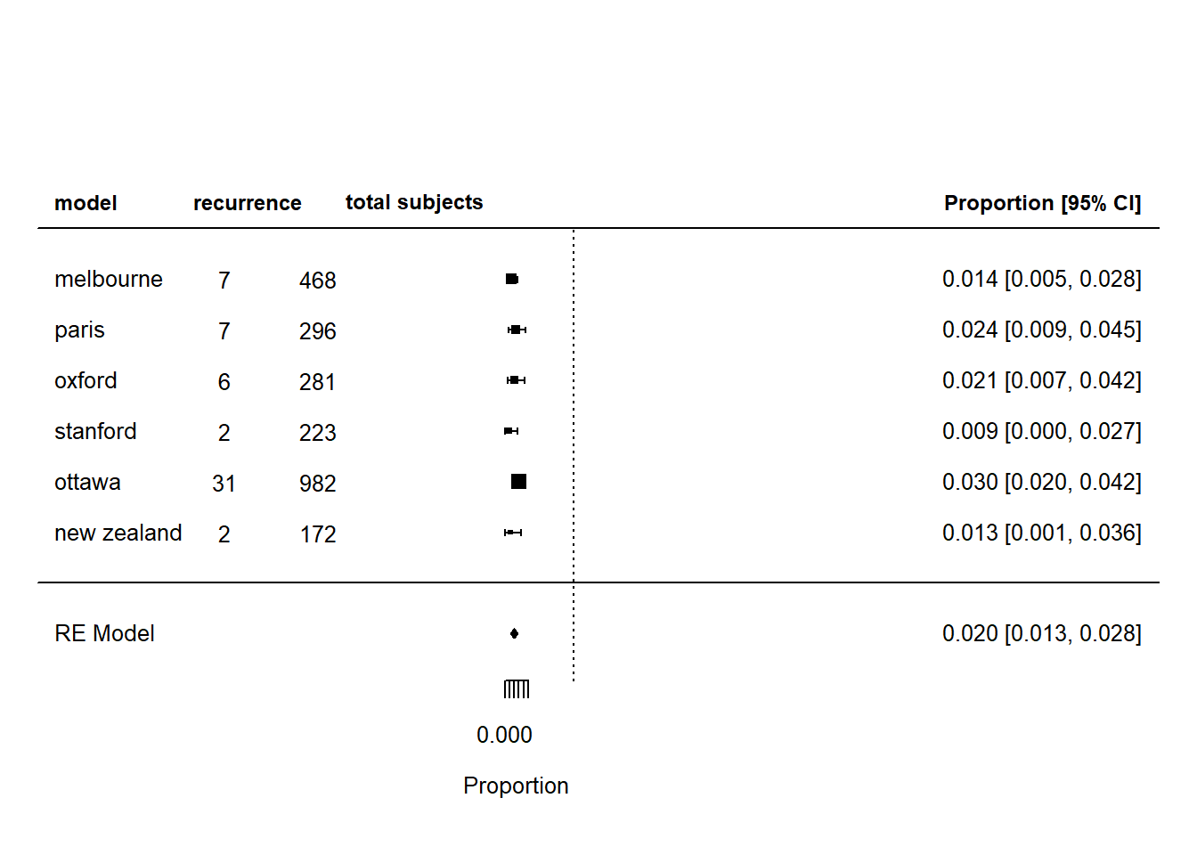
par(op)Exact 95% confidence interval for proportion is provided below using the TIA data above. This solution was provided on stack overflow. This is performed using the binomial.test function.
#exact confidence interval
sapply(split(dat, dat$model),
       function(x) binom.test(x$xi, x$ni)$conf.int)
melbourne new zealand ottawa oxford paris stanford
[1,] 0.00603419 0.001411309 0.02154780 0.007875285 0.00955965 0.001087992
[2,] 0.03057375 0.041370853 0.04451101 0.045893259 0.04811612 0.032020390The data needs to be transposed using t function. This generates one column for lower and another for upper CI. Note that sapply returns a matrix or array and the column names have to be assigned.
#the data
tmp <- t(sapply(split(dat, dat$model),
                function(x) binom.test(x$xi, x$ni)$conf.int))
tmp
[,1] [,2]
melbourne 0.006034190 0.03057375
new zealand 0.001411309 0.04137085
ottawa 0.021547797 0.04451101
oxford 0.007875285 0.04589326
paris 0.009559650 0.04811612
stanford 0.001087992 0.03202039The exact confidence is now put back into the _dat_ data frame.
dat$ci.lb <- tmp[,1] #adding column to data frame dat
dat$ci.ub <- tmp[,2] #adding column to data frame dat

dat <- escalc(measure="PFT", xi=xi, ni=ni, data=dat, add=0)
res <- rma.glmm(measure="PLO", xi=xi, ni=ni, data=dat)


#insert the exact confidence interval
with(dat, metafor::forest(yi, ci.lb=ci.lb, ci.ub=ci.ub,
  ylim=c(-1.5,8.5),
  xlim=c(-1.1,1),
  refline=predict(res, transf=transf.ilogit)$pred,
  cex=.8,
  ilab=cbind(dat$xi, dat$ni),
  ilab.xpos=c(-.6,-.2),digits=3))

op <- par(cex=.75, font=2)
addpoly(res, row=-1, transf=transf.ilogit)
abline(h=0)
#position of column names on x-axis
text(-.9, 7.5, "Model", pos=2)
text(c(-.55,-.2), 7.5, c("recurrence", " total subjects"))
text( 1,   7.5, "Proportion [95% CI]", pos=2)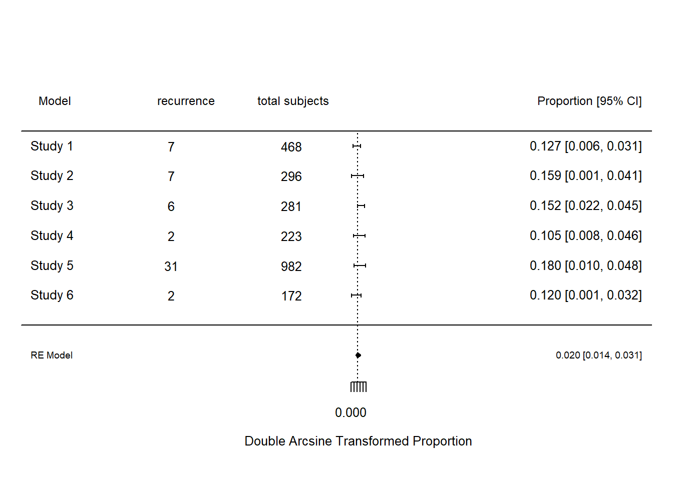
7.0.5.1 Summary Positive and Negative Likelihood Ratio
Positive likelihood ratio (PLR) is the ratio of sensitivity to false positive rate (FPR); the negative (NLR) likelihood ratio is the ratio of 1-sensitivity to specificity. A PLR indicates the likelihood that a positive spot sign (test) would be expected in a patient with target disorder compared with the likelihood that the same result would be expected in a patient without target disorder. Using the recommendation by Jaeschke et al(Jaeschke, Guyatt, and Sackett 1994) a high PLR (>5) and low NLR (<0.2) indicate that the test results would make moderate changes in the likelihood of hematoma growth from baseline risk. PLRs of >10 and NLRs of <0.1 would confer very large changes from baseline risk. The pooled likelihood ratios were used to calculate post-test odds according to Bayes’ Theorem and post-test probabilities of outcome after a positive test result for a range of possible values of baseline risk.
7.0.5.1.1 Fagan’s normogram
Data from likelihood ratio can be used to create Fagan’s normogram.
#The code for this is available at
#"https://raw.githubusercontent.com/achekroud/nomogrammer/master/nomogrammer.r"
library(nomogrammer)
p<-nomogrammer(Prevalence = .234, Plr = 4.85, Nlr = 0.49)
p+ggtitle("Fagan's normogram for Spot Sign and ICH growth")

#ggsave(p,file="Fagan_SpotSign.png",width=5.99,height=3.99,units="in")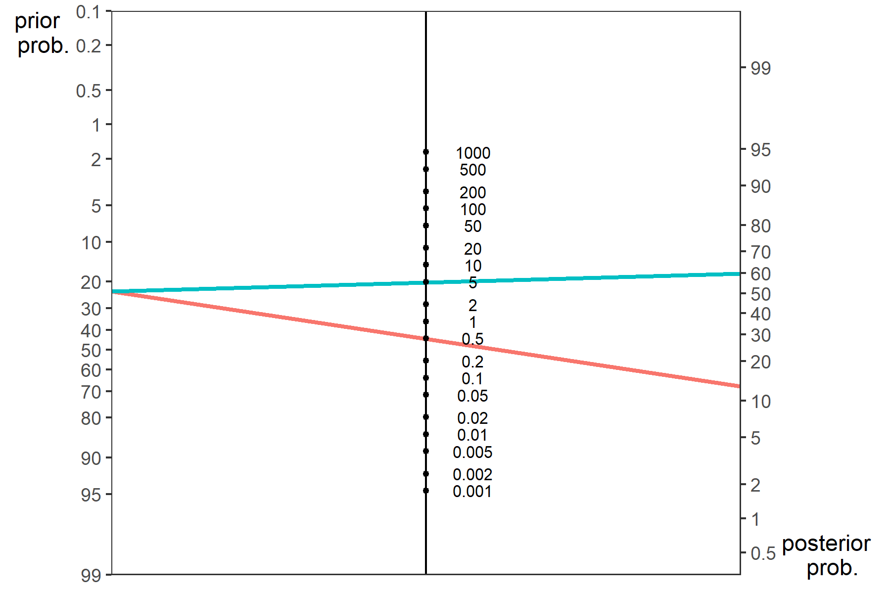
7.0.6 Metaanalysis of continuous data
Metanalysis of continuous outcome data can be performed using standardised mean difference or ratio of means. It is available in the meta library using metacont function (Balduzzi, Rücker, and Schwarzer 2019).
7.0.7 Univariate metaanalysis
The univariate method of Moses-Shapiro-Littenberg combines these measures (sensitivity and specificity) into a single measure of accuracy (diagnostic odds ratio)(Moses, Shapiro, and Littenberg 1993) .
7.0.7.1 Summary ROC
The summary ROC curve summarises the central tendency of the ROC of the various studies for a given test (Moses, Shapiro, and Littenberg 1993). The diagnostic OR is related to AUC of summary ROC (SD 2002).
\(AUC=\int_0^1 \frac{1}{1+\frac{1}{DiagnosticOR*(\frac{x}{1-x})}}dx\)
When the diagnostic OR is 1, the AUC is 0.5. A diagnostic OR of 2 corresponds to AUC of 0.61, diagnostic OR of 5 corresponds to AUC 0.75 and diagnostic OR of 10 correspond to AUC of 0.83. The diagnostic OR is related to PLR and NLR.
\(Diagnostic OR=\frac{PLR}{NLR}\)
7.0.8 Bivariate Metaanalysis
This Moses-Shapiro-Littenberg approach has been criticized for losing data on sensitivity and specificity of the test.(Moses, Shapiro, and Littenberg 1993) . Similar to the univariate method, the bivariate method employs a random effect to take into account the within study correlation (Reitsma et al. 2005). Additionally, the bivariate method also accounts for the between-study correlation in sensitivity and specificity. Bivariate analysis is performed using mada package. A Bayesian method for bivariate analysis meta4diag is under Bayesian analysis chapter.
The example below is taken from a metaanalysis of spot sign as predictor expansion of intracerebral hemorrhage (Phan et al. 2019). The data for this analysis is available in the Data-Use sub-folder.
library(mada)Loading required package: mvtnormLoading required package: ellipse
Attaching package: 'ellipse'The following object is masked from 'package:graphics':
pairsLoading required package: mvmetaThis is mvmeta 1.0.3. For an overview type: help('mvmeta-package').
Attaching package: 'mvmeta'The following object is masked from 'package:metafor':
blupThe following object is masked from 'package:meta':
blup
Attaching package: 'mada'The following object is masked from 'package:metafor':
forestThe following object is masked from 'package:meta':
forest#spot sign data
Data<-read.csv("./Data-Use/ss150718.csv")
#remove duplicates using subset
#another way is to use filter from dplyr
Dat<-subset(Data, Data$retain=="yes")
(ss<-reitsma(Dat))Call: reitsma.default(data = Dat)
Fixed-effects coefficients:
tsens tfpr
(Intercept) 0.2548 -1.9989
27 studies, 2 fixed and 3 random-effects parameters
logLik AIC BIC
52.0325 -94.0650 -84.1201 summary(ss)Call: reitsma.default(data = Dat)
Bivariate diagnostic random-effects meta-analysis
Estimation method: REML
Fixed-effects coefficients
Estimate Std. Error z Pr(>|z|) 95%ci.lb 95%ci.ub
tsens.(Intercept) 0.255 0.152 1.676 0.094 -0.043 0.553 .
tfpr.(Intercept) -1.999 0.097 -20.664 0.000 -2.189 -1.809 ***
sensitivity 0.563 - - - 0.489 0.635
false pos. rate 0.119 - - - 0.101 0.141
---
Signif. codes: 0 '***' 0.001 '**' 0.01 '*' 0.05 '.' 0.1 ' ' 1
Variance components: between-studies Std. Dev and correlation matrix
Std. Dev tsens tfpr
tsens 0.692 1.000 .
tfpr 0.400 -0.003 1.000
logLik AIC BIC
52.033 -94.065 -84.120
AUC: 0.858
Partial AUC (restricted to observed FPRs and normalized): 0.547
I2 estimates
Zhou and Dendukuri approach: 10.2 %
Holling sample size unadjusted approaches: 64.2 - 79.9 %
Holling sample size adjusted approaches: 4.7 - 5 %AUC(reitsma(data = Dat))$AUC
[1] 0.8576619
$pAUC
[1] 0.5474316
attr(,"sroc.type")
[1] "ruttergatsonis"sumss<-SummaryPts(ss,n.iter = 10^3) #bivariate pooled LR
summary(sumss) Mean Median 2.5% 97.5%
posLR 4.720 4.730 3.730 5.760
negLR 0.498 0.498 0.415 0.585
invnegLR 2.020 2.010 1.710 2.410
DOR 9.620 9.520 6.600 13.200A more elegant way to perform this type of analysis is to use iteration concept with the map function from the purr library. This was illustrated in the Data Wrangling chapter whereby the data was split and the regression of sensitvity and Year of publication was performed within this iteration.
7.0.9 Metaanalysis of clinical trial.
Fixed effect (Peto or Mantel-Haenszel) approaches assume that the population is the same for all studies and thus each study is the source of error. Random effect (DerSimonian Laird) assumes an additional source of error between studies.The random effect approach results in more conservate estimate of effect size confidence interval. A criticism of DerSimnonian and Laird approach is that it is prone to type I error especially when the number of number of studies is small (n<20) or moderate heterogeneity. It’s estimated that 25% of the significant findings with DerSimonian Laird method may be non-significant with Hartung-Knapp method (BMC Medical Research Methodology 2014, 14:25). The Hartung-Knapp method (Stat Med 2001;20:3875-89) estimate the between studies variance and treat it as fixed. It employs quantile of t-distribution rather than normal distribution. The Hartung-Knapp method is available in meta and metafor package.
The data is from Jama Cardiology on Associations of Omega-3 Fatty Acid Supplement Use With Cardiovascular Disease Risks Meta-analysis of 10 Trials Involving 77917 Individuals (Aung T 2018). Subsequently a meta-analysis (Hu 2019) reported that contrary to the earlier meta-analysis, Omega-3 lowers the risk of cardiovascular diseases with effect related to dose. The analysis using DerSimonian Laird and Hartung Knapp method is illustrated below.
library(tidyverse)── Attaching core tidyverse packages ──────────────────────── tidyverse 2.0.0 ──
✔ dplyr 1.1.2 ✔ readr 2.1.4
✔ forcats 1.0.0 ✔ stringr 1.5.0
✔ ggplot2 3.5.1 ✔ tibble 3.2.1
✔ lubridate 1.9.2 ✔ tidyr 1.3.0
✔ purrr 1.0.1
── Conflicts ────────────────────────────────────────── tidyverse_conflicts() ──
✖ tidyr::expand() masks Matrix::expand()
✖ dplyr::filter() masks stats::filter()
✖ dplyr::lag() masks stats::lag()
✖ tidyr::pack() masks Matrix::pack()
✖ readr::spec() masks mada::spec()
✖ tidyr::unpack() masks Matrix::unpack()
ℹ Use the conflicted package (<http://conflicted.r-lib.org/>) to force all conflicts to become errorslibrary(metafor)
#Omega 3 data
Year=c(2010,2014,2010,2007,2010,2010,2013,2008,2012,1999)
Trials=c("DOIT","AREDS-2","SU.FOL.OM3","JELIS","Alpha Omega","OMEGA","R&P","GISSI-HF","ORIGIN","GISSI-P")
Treatment=c(29,213,216,262,332,534,733,783,1276,1552)
Treatment.per=c(10.3,9.9,17.2,2.8,13.8,27.7,11.7,22.4,20.3,27.4)
Control=c(35,208,211,324,331,541,745,831,1295,1550)
Control.per=c(12.5,10.1,16.9,3.5,13.6,28.6, 11.9,23.9,20.7,27.3)
#combine into data frame
rct<-data.frame(Year,Trials,Treatment,Treatment.per,Control,Control.per) %>%
mutate(Treatment.number=round(Treatment*100/Treatment.per,0),
Control.number=round(Control*100/Control.per,0), group=ifelse(Year>2010,"wide","narrow")) %>%
rename(ai=Treatment,n1i=Treatment.number,ci=Control,
n2i=Control.number,study=Trials)
#peto's fixed effect method
res <- rma.peto(ai=ai, n1i=n1i, ci=ci, n2i=n2i, data=rct)
print(res, digits=2)
Equal-Effects Model (k = 10)

I^2 (total heterogeneity / total variability):  0.00%
H^2 (total variability / sampling variability): 0.93

Test for Heterogeneity:
Q(df = 9) = 8.36, p-val = 0.50

Model Results (log scale):

estimate    se   zval  pval  ci.lb  ci.ub
   -0.04  0.02  -1.72  0.08  -0.08   0.00

Model Results (OR scale):

estimate  ci.lb  ci.ub
0.97 0.93 1.00 result<-predict(res, transf=exp, digits=2)
#forest plot
metafor::forest(res, targs=list(study=rct$study),
main="RCT of Omega3 fatty acid for cardiovascular disease-Peto")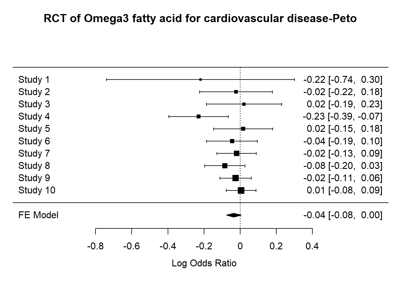
The funnel plot is used here to illustrate presence or absence publication bias. In this case the funnel plot reflects the same findings as the low \(I^2\) value. There is one outlier. We will explore this further with the GOSH plot below.
# funnel plot
funnel(res, refline=0,
       level=c(90, 95, 99),
shade=c("white", "gray", "darkgray")) 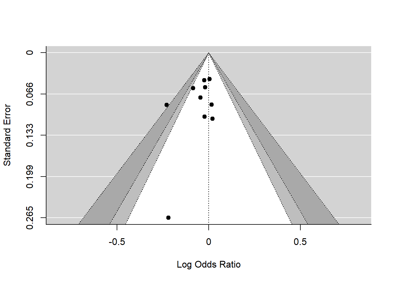
Random effect (DerSimonian Laird) assumes an additional source of error between studies when calculating odds ratio.
#DL
datO3 <- escalc(measure = "OR",ai=ai, n1i=n1i, ci=ci, n2i=n2i,
                data=rct)
res.DL<-rma(yi,vi, method = "DL",data=datO3)

metafor::forest(res.DL,
    main="RCT of Omega3 fatty acid for cardiovascular disease-DL")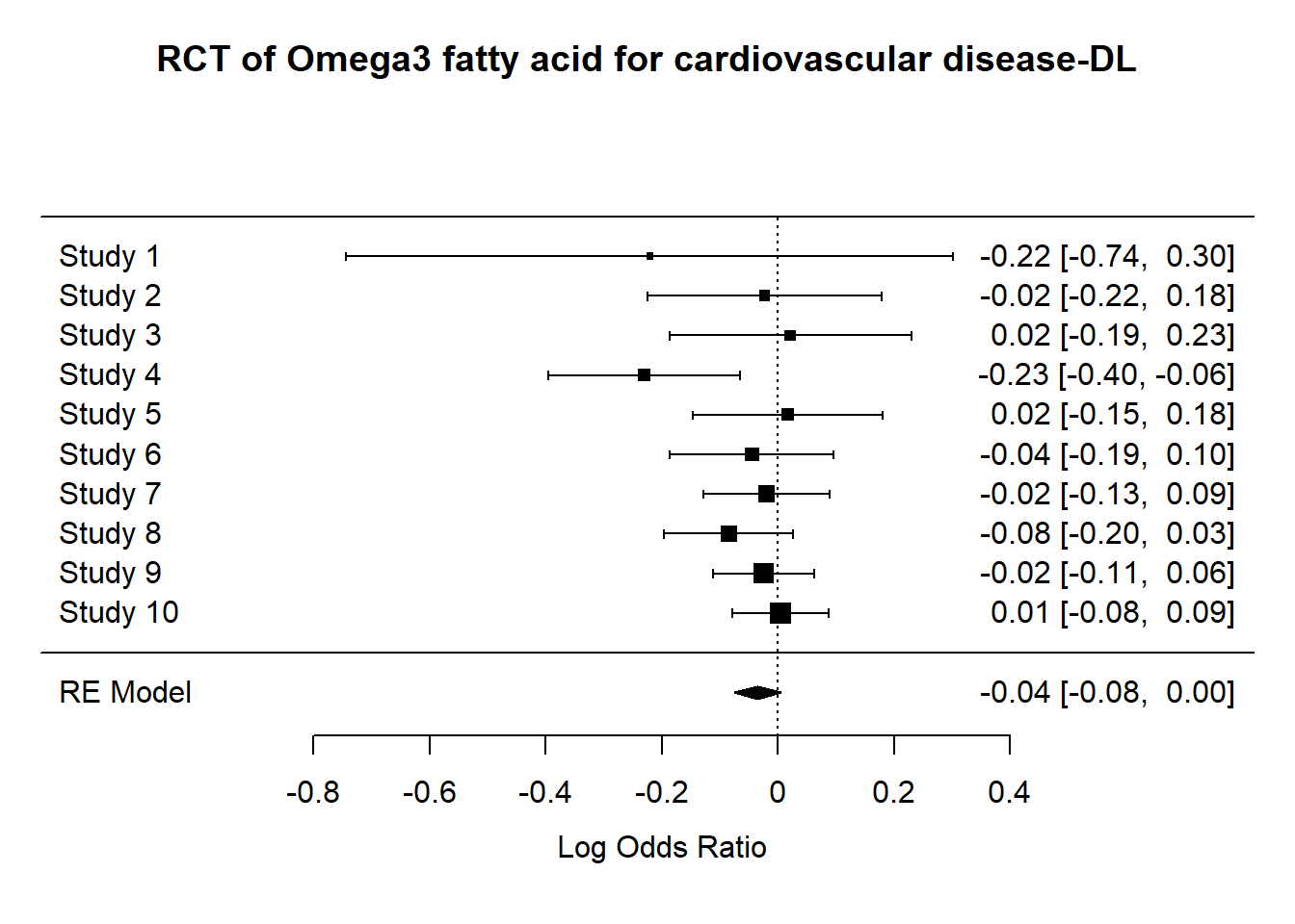
7.0.9.1 Hartung Knapp random effect
DerSimonian Laird method may not be appropriate for metaanalysis with small number of studies . The recommendation is to use the Hartung Knapp random effect method. This analysis show that inspite of the small sample size the significant findings remain.
#Hartung-ignore error message
res.HK<-rma.uni(yi,vi=1/vi,method="FE",knha=TRUE,data=datO3)

metafor::forest(res.HK,
    main="RCT of Omega3 fatty acid for cardiovascular disease-HK")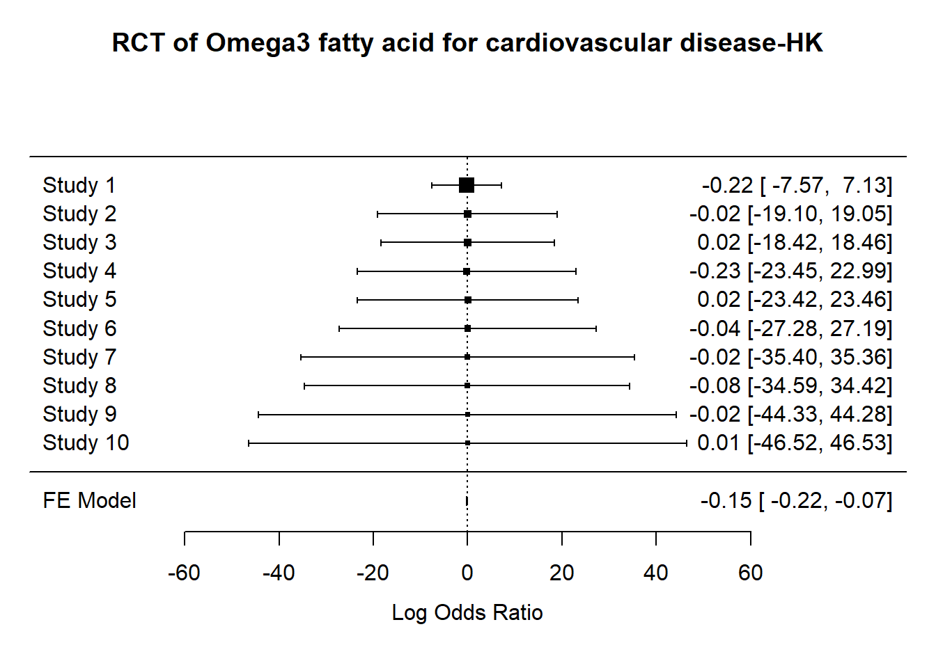
Subgroup analysis is one way of exploring the data for group effect. Metaregression is illustrated later.
#datO3$group<-rct3$group
#plot subgroups
res.group <- rma(yi, vi, mods = ~ group, data=datO3)
res.wide<- rma(yi, vi, subset=(group=="wide"), data=datO3)
res.wide
res.narrow<- rma(yi, vi, subset=(group=="narrow"), data=datO3)
res.narrow
#https://stackoverflow.com/questions/39392706/using-the-r-forestplot-package-
#is-there-a-way-to-assign-variable-colors-to-boxe

#confidence interval
rmeta_conf <-
  structure(list(
    mean  = c(NA, NA, exp(-0.0676), exp(-0.0266),  NA, exp(-0.0352)),
    lower = c(NA, NA, exp(-0.1873), exp(-0.0715),  NA, exp(-0.0753)),
    upper = c(NA, NA, exp(0.0520), exp(0.0183),  NA, exp(0.0049))),
    .Names = c("mean", "lower", "upper"),
    row.names = c(NA, -6L),
    class = "data.frame")

#table data
tabletext<-cbind(c("","Trials","wide","narrow",NA,"Summary"),
    c("Events","(Drugs)",sum(filter(datO3,group=="wide")$ai),
      sum(filter(datO3,group=="narrow")$ai),NA,NA),
    c("Events","(Control)",sum(filter(datO3,group=="wide")$ci),
      sum(filter(datO3,group=="narrow")$ci),NA,NA),
    c("","OR","0.934","0.974",NA,"0.965")
                 )
#use forestplot as another library to perform forest plot
library(forestplot)
 forestplot(tabletext,
       rmeta_conf,new_page = TRUE,
       is.summary=c(TRUE,TRUE,rep(FALSE,8),TRUE),
       clip=c(0.1,2.5),
       xlog=TRUE,
       col=fpColors(box="royalblue",line="darkblue", summary="royalblue"))
Baujat plot is another method in addition to funnel plot explore heterogeneity
# adjust margins so the space is better used
par(mar=c(5,4,2,2)) # create Baujat plot to explore source of heterogeneity
baujat(res.DL, xlim=c(0,20), ylim=c(0,0.2))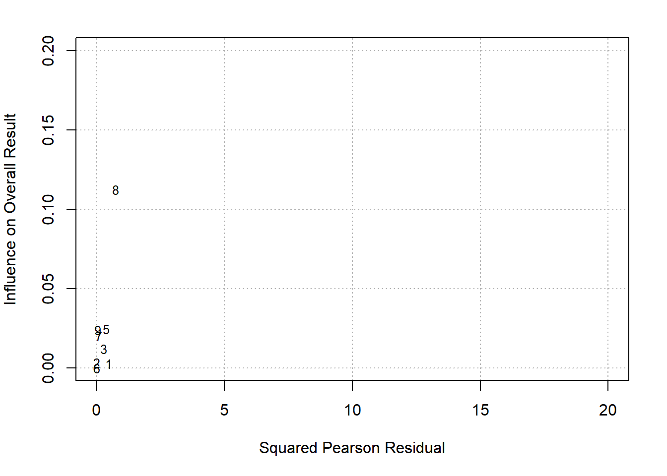
GOSH plot explores study heterogeneity using output of fixed effect model for all possible subsets
## fit FE model to all possible subsets # uses output from DL analysis
sav <- gosh(res.DL)
Fitting 1023 models (based on all possible subsets).### create GOSH plot
### red points for subsets that include and blue points
### for subsets that exclude study 16 (the ISIS-4 trial)
plot(sav, out=dim(rct)[1], breaks=100) 
7.0.9.2 Network metaanalysis
Network metaanalysis provides an indirect method to compare different therapies. This method rank treatments using a probability measure called surface under the cumulative rank curve (SUCRA). This measure is the probability that a treatment is the best option among those tested. (Lim, Ma, Ly, et al. 2024). One R library is the Bayesian NMA with the BUGSnet (Bayesian Inference Using Gibbs Sampling to Conduct an NMA) and JAGS (Just Another Gibbs Sampler) packages. The BUGSnet library is recommended for NMA because it provides the necessary output required by various societies including the International Society of Pharmacoeconomics and Outcomes–Academy of Managed Care Pharmacy–National Pharmaceutical Council.
7.0.10 Metaregression
Metaregression is used to explain heterogeneity in the data. This is first done for tsens
#separate metaregression for tsens and tfpr

#tsens - setting single or multicentre for spot sign metaanalysis
dat1<-subset(Dat, Dat$result_id==1 )
(metass<-reitsma(dat1, formula = cbind(tsens,tfpr)~PubYear+Study.type+Setting+Quality.assessment))
Call: reitsma.default(data = dat1, formula = cbind(tsens, tfpr) ~ PubYear +
Study.type + Setting + Quality.assessment)
Fixed-effects coefficients:
tsens tfpr
(Intercept) 298.7348 -164.8603
PubYear -0.1484 0.0828
Study.typeRetro 0.3554 -0.1489
SettingSingle 0.2283 -0.1301
Quality.assessment -0.0040 -0.0834
26 studies, 10 fixed and 3 random-effects parameters
logLik AIC BIC
48.5386 -71.0771 -45.7109 summary(metass)Call: reitsma.default(data = dat1, formula = cbind(tsens, tfpr) ~ PubYear +
Study.type + Setting + Quality.assessment)
Bivariate diagnostic random-effects meta-regression
Estimation method: REML
Fixed-effects coefficients
Estimate Std. Error z Pr(>|z|) 95%ci.lb 95%ci.ub
tsens.(Intercept) 298.735 143.547 2.081 0.037 17.387 580.083
tsens.PubYear -0.148 0.071 -2.078 0.038 -0.288 -0.008
tsens.Study.typeRetro 0.355 0.310 1.146 0.252 -0.253 0.963
tsens.SettingSingle 0.228 0.495 0.462 0.644 -0.741 1.198
tsens.Quality.assessment -0.004 0.050 -0.081 0.936 -0.102 0.094
tfpr.(Intercept) -164.860 80.574 -2.046 0.041 -322.783 -6.938
tfpr.PubYear 0.083 0.040 2.066 0.039 0.004 0.161
tfpr.Study.typeRetro -0.149 0.172 -0.865 0.387 -0.486 0.188
tfpr.SettingSingle -0.130 0.276 -0.471 0.638 -0.672 0.412
tfpr.Quality.assessment -0.083 0.026 -3.190 0.001 -0.135 -0.032
tsens.(Intercept) *
tsens.PubYear *
tsens.Study.typeRetro
tsens.SettingSingle
tsens.Quality.assessment
tfpr.(Intercept) *
tfpr.PubYear *
tfpr.Study.typeRetro
tfpr.SettingSingle
tfpr.Quality.assessment **
---
Signif. codes: 0 '***' 0.001 '**' 0.01 '*' 0.05 '.' 0.1 ' ' 1
Variance components: between-studies Std. Dev and correlation matrix
Std. Dev tsens tfpr
tsens 0.657 1.000 .
tfpr 0.297 0.312 1.000
logLik AIC BIC
48.539 -71.077 -45.711
I2 estimates
Zhou and Dendukuri approach: 0 %
Holling sample size unadjusted approaches: 66.8 - 80.5 %
Holling sample size adjusted approaches: 5.4 - 5.8 %Plot year against tsens from metaregression
#using output from spot sign

library(ggplot2)
library(lubridate)
ssr<-as.data.frame(ss$residuals)
#convert character to year
ssr$Year<-as.Date(as.character(Dat$PubYear),"%Y")
ssr$Quality<-Dat$Quality.assessment
ggplot(ssr, aes(x=ssr$Year,y=ssr$tsens))+geom_point()+
  scale_x_date()+geom_smooth(method="lm")+
  ggtitle("Relationship between transformed sensitivity and Publication Year")+
  labs(x="Year",y="transformed sensitivity")
`geom_smooth()` using formula = 'y ~ x'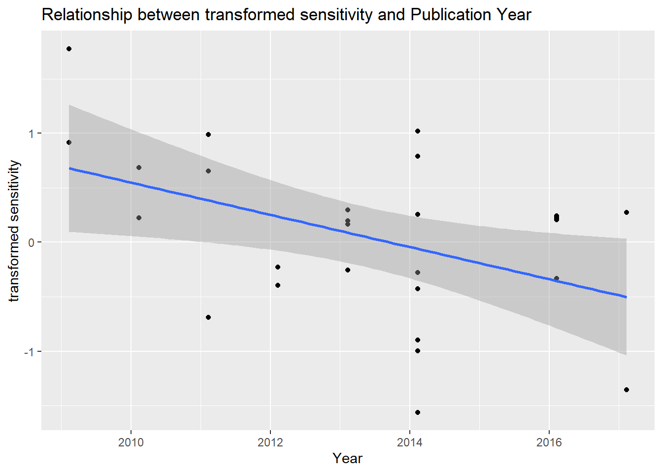
Metaregression is performed for tfpr.
#tfpr - setting single or multicentre for spot sign metaanalysis

dat1<-subset(Dat, Dat$result_id==1 )

(metassfull<-reitsma(dat1, formula = cbind(tsens,tfpr)~         PubYear+clinical+Study.type+CTA6hrs+Setting+Quality.assessment))
Call: reitsma.default(data = dat1, formula = cbind(tsens, tfpr) ~ PubYear +
clinical + Study.type + CTA6hrs + Setting + Quality.assessment)
Fixed-effects coefficients:
tsens tfpr
(Intercept) 297.5416 -144.2754
PubYear -0.1480 0.0724
clinical -0.4703 -0.1810
Study.typeRetro 0.4884 -0.0989
CTA6hrsyes -0.2141 -0.2342
SettingSingle 0.2568 -0.1435
Quality.assessment 0.0130 -0.0738
26 studies, 14 fixed and 3 random-effects parameters
logLik AIC BIC
48.4477 -62.8955 -29.7243 summary(metassfull)Call: reitsma.default(data = dat1, formula = cbind(tsens, tfpr) ~ PubYear +
clinical + Study.type + CTA6hrs + Setting + Quality.assessment)
Bivariate diagnostic random-effects meta-regression
Estimation method: REML
Fixed-effects coefficients
Estimate Std. Error z Pr(>|z|) 95%ci.lb 95%ci.ub
tsens.(Intercept) 297.542 150.543 1.976 0.048 2.482 592.601
tsens.PubYear -0.148 0.075 -1.977 0.048 -0.295 -0.001
tsens.clinical -0.470 0.333 -1.411 0.158 -1.124 0.183
tsens.Study.typeRetro 0.488 0.321 1.523 0.128 -0.140 1.117
tsens.CTA6hrsyes -0.214 0.322 -0.665 0.506 -0.845 0.417
tsens.SettingSingle 0.257 0.495 0.519 0.604 -0.714 1.228
tsens.Quality.assessment 0.013 0.051 0.255 0.799 -0.087 0.113
tfpr.(Intercept) -144.275 82.720 -1.744 0.081 -306.403 17.852
tfpr.PubYear 0.072 0.041 1.761 0.078 -0.008 0.153
tfpr.clinical -0.181 0.187 -0.969 0.333 -0.547 0.185
tfpr.Study.typeRetro -0.099 0.177 -0.558 0.577 -0.446 0.249
tfpr.CTA6hrsyes -0.234 0.177 -1.322 0.186 -0.581 0.113
tfpr.SettingSingle -0.144 0.274 -0.524 0.600 -0.680 0.393
tfpr.Quality.assessment -0.074 0.027 -2.774 0.006 -0.126 -0.022
tsens.(Intercept) *
tsens.PubYear *
tsens.clinical
tsens.Study.typeRetro
tsens.CTA6hrsyes
tsens.SettingSingle
tsens.Quality.assessment
tfpr.(Intercept) .
tfpr.PubYear .
tfpr.clinical
tfpr.Study.typeRetro
tfpr.CTA6hrsyes
tfpr.SettingSingle
tfpr.Quality.assessment **
---
Signif. codes: 0 '***' 0.001 '**' 0.01 '*' 0.05 '.' 0.1 ' ' 1
Variance components: between-studies Std. Dev and correlation matrix
Std. Dev tsens tfpr
tsens 0.650 1.000 .
tfpr 0.285 0.188 1.000
logLik AIC BIC
48.448 -62.895 -29.724
I2 estimates
Zhou and Dendukuri approach: 0 %
Holling sample size unadjusted approaches: 66.8 - 80.5 %
Holling sample size adjusted approaches: 5.4 - 5.8 %7.0.10.1 Combining data from RCT and observational studies
The issue regarding combining data from RCT and observational studies in the setting of an intervention is complex (AM J Epidemiol 2007;166:1203–1209 and N Engl J Med 2000; 342:1887-1892). Some investigators argued that inclusion of well conducted observational studies is appropriate. One way to resolve this issue is to perform multilevel random‐effects meta‐analysis with grouping of the type of study (Lim, Ma, Johnston, et al. 2024).